Different models of computation are used in different phases of a design process. We discuss the suitability of MoCs in three design activities.
Performance analysis aims to assess and understand some quantitative properties at an early stage of the product development. As examples we take buffer analysis and delay analysis and find that the U-MoC is suitable for many performance analysis tasks as long as no timing information is required. Buffer analysis is a good case in point. When timing information is required, a synchronous or timed MoC should be used. For many time-related analysis tasks a synchronous MoC is sufficient. A timed MoC is the most general tool and should be used only when a synchronous MoC is not sufficiently accurate.
The functional specification document is used for two, partly contradictory, purposes. On the one hand, a functional model should reflect the first high-level solution to the posed problem. It should help to assess the quality adequacy of this solution. On the other hand, it is the basis for the next design steps and the implementation. As such it should help to assess the feasibility of the solution and its performance and cost properties. Based on an analysis of the objectives of the functional specification, we conclude all three MoCs may be required, but the synchronous MoC is appropriate for most tasks.
In synthesis and design all three MoCs are required. The closer we come to the final implementation, the more accurate the timing information should be. Thus, we see a refinement from an untimed into a synchronous into a timed MoC. Not surprisingly, the general rule is to avoid detailed timing information as long as possible and to use a more accurate timing model whenever necessary.
In the previous chapters we reviewed several important models of computation and concurrency and discussed some of their essential features. On several occasions we have related these features to applications of modeling. For instance, we found that discrete event models are very good for capturing and simulating the accurate timing behavior of existing systems, but they are ill suited to serve as an entry point for synthesis and formal verification tasks. The discussion should have made clear by now that features of computational models are not good or bad, but they are merely more or less useful for a particular purpose.
In this chapter we consider some important applications of modeling, and we shall analyze their requirements on models in a more systematic way. We will find out that even within the same application area some requirements contradict each other. For instance, system specification serves essentially two different purposes: capturing the system functionality and forming the basis for design and implementation. However, requirements derived from these two purposes contradict each other directly to some degree. On the one hand, the system specification model should be as abstract and application oriented as possible to allow an implementation-independent exploration of system features and for a solid basis for contacts with the application-oriented customer. On the other hand, it should be implementation sensitive to allow accurate performance and cost estimation and to have a good starting point for an efficient design and implementation process.
The contradictions between different application areas such as performance modeling and synthesis are insurmountable. Therefore we have a variety of computational models with different features, strengths, and weaknesses.
We have selected some of the most important applications. No larger system design project can avoid any of these. But by no means can we cover all application areas of interest. For instance we do not touch upon the equally important fields of requirements engineering and the modeling and design of analog components. Moreover, we do not attempt an in-depth treatment of the application areas that we do take up. We do not present a thorough account of the theory and techniques of performance modeling or formal verification. Numerous good books are devoted solely to these subjects. We provide a rather superficial introduction to these topics with the objective of extracting and explicitly discussing the requirements and constraints they impose on modeling concepts and techniques. We summarize the requirements from different applications and discuss them in light of the computational models we have available. From this discussion we will obtain a better understanding of what a computational model can accomplish and which model we should select for a given task.
It will also allow us to relate modeling concepts in a different way. In the previous chapter we categorized them with the help of the Rugby metamodel based on the purely technical feature of abstraction levels in different domains. Now we relate them in terms of appropriateness in the context of given tasks and applications. We will notice that there is a certain correlation between the two points of view because specific applications tend to be concerned with only certain abstraction levels. For instance, performance modeling almost exclusively deals with data at the Symbol and Number level. We shall investigate this correlation briefly and also examine how it relates to typical design phases in development projects.
System performance is as important as functionality. The term “performance” is used with two different meanings. In its narrower sense it denotes time behavior, for example, how fast the system can react to events, at which period it can process input signals. In its broader sense it also includes many other nonfunctional properties such as acceptable noise levels of input signals, mean time between failures, reliability, fault tolerance, and other parameters. It is typically limited to properties that can be measured and quantified and does not include features such as “convenience of use.” Hence, the terms “performance analysis” and “performance modeling” are restricted to a numerical analysis of some sort.
In general we always prefer closed formulas based on a mathematical model that describes the parameters of interest. For instance, E[X] = λE[S] tells us how the mean queue length E[X] depends on the mean customer arrival rate λ and the mean system processing time E[S] of an arbitrary system. This equation, known as Little’s law, is very general and useful because it allows us to dimension system buffers without knowing many of the details such as the scheduling policy of incoming customers, the number and organization of buffers, the number and operation of service units, precise sequence and timing of input events, and so on. Based on a measurement of the mean time of input events and knowing Little’s law, we can dimension the input buffers with respect to an expected system timing performance, or we can decide on the buffer sizes and formulate performance requirements for the system design and implementation.
Unfortunately, closed formulas are the exception rather than the rule. Either we do not have suitable mathematical models of the concerned properties that allow us to derive closed formulas, or the formulas are complex differential or difference equations that, in general, cannot be solved accurately. In these cases we have to resort to simulation as the only universally applicable tool of analysis. The main drawback of simulation is that the result depends on the selected inputs. Typically we can only apply a tiny fraction of the total input space in a simulation, which makes the result sensitive to the quality of the inputs.
We restrict the discussion to the buffer size analysis and delay analysis by using the untimed and the synchronous MoC, respectively.
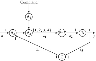
Consider the process network in Figure 9-1 with three processes, A, B, and C. The numbers at the inputs and outputs of the processes denote the number of tokens a process consumes and produces at each invocation. Thus, process B reads one token from its input and emits one token to each of its outputs. Process A can emit one, two, three, or four tokens, depending on its state, which is controlled by the command input. In state α the process always emits one token, in state β it emits one token in 99.5% of the invocations and two tokens in 0.5%, in state γ it emits three tokens in 0.5% of its invocations, and in state δ four tokens in 0.5% of invocations. Commands from the command input set the state of the process. If we assume that all processes need equally long for each invocation, a simple analysis reveals that if process A is in state α, the system is in a steady state without the need for internal buffers. On the other hand, when process A is in one of the other states, it produces more tokens than B can consume, and any finite-size buffer between A and B will eventually overflow.

Let us further assume we are dealing with some kind of telecommunication network that receives, transforms, and emits communication packets. State α is the normal mode of operation that is active most of the time. However, occasionally the system is put into a monitoring mode, for instance, to measure the performance of the network and identify broken nodes. Monitoring packets are sent out to measure the time until they arrive at a specific destination node, and to count how many are lost along the way. A monitoring phase runs through the following sequence of states: state β for 1000 tokens, state γ for 1000 tokens, state δ for 1000 tokens, state γ for 1000 tokens, and finally state β for 1000 tokens before state α is resumed again. Even if we introduce a buffer between A and B to handle one monitoring phase, the system would still be instable because the system is running under full load even in state α and cannot reduce the number of packets in the buffer between the monitoring phases. Consequently, a finite-size buffer would still overflow if we run the monitoring phases often enough.
To make the example more interesting and realistic, we also make some assumptions about the traffic and how it is processed. Some of the packets are in fact idle packets, which only keep the nodes synchronized and can be dropped and generated as needed. The packets are represented as integers, and idle packets have the value 0. Processes B and C pass on the packets unchanged, but A processes the packets according to the formula z = (x + y) mod 100, where x and y are input packets and z is the output packet. Consequently, packet values at the output of A are confined to the range 0 ... 99.
To handle the monitoring phases, we introduce a buffer between processes A and B that drops idle packets when they arrive and emits idle packets when the buffer is empty and process B requests packets. What is the required buffer size?
Apparently, the answer depends on the characteristics of the input traffic, and in particular how many idle cells there are. Let m be the number of excess packets per normal input packet, introduced by a monitoring process, i is the fraction of idle packets, and N is the total number of input packets in the period we consider. In the first step of the monitoring phase, where process A is in state β, we have

The number of packets we have to buffer is the number of excess packets, introduced by the monitoring activity, minus the number of idle packets:
We need the max function because B may never become negative; that is, the number of buffered packets cannot be less than 0. For the entire monitoring phase we get
m | N | |
|---|---|---|
state β | 0.005 | 2000 |
state γ | 0.01 | 2000 |
state δ | 0.015 | 1000 |
If we assume a uniform distribution of input packet types, only 1% of the input packets are idle packets, and according to (9.1) we get
B | = | max(0, 0.005 − 0.01) · 1000 + max(0, 0.01 − 0.01) · 1000 |
+ max(0, 0.015 − 0.01) · 1000 + max(0, 0.01 − 0.01) · 1000 | ||
+ max(0, 0.005 − 0.01) · 1000 | ||
= | 5 |
Only state δ seems to require buffering, and a buffer of size 5 would suffice to avoid a loss of packets. However, (9.1) assumes that the excess and idle packets are evenly distributed over the considered period of N packets. This is not correct; excess packets come in bursts of 1, 2, or 3 at a time, rather than 0.005 at a time. Thus, even in state β the buffer has to be prepared to handle the bursts, until consecutive idle packets allow the buffer to empty again. Consequently, we modify (9.1) to take bursts into account, with b denoting the longest expected bursts of excess packets:
For the entire monitoring phase we get
B | = | max(0, 0.005 – 0.01) · 1000 + 1 + max(0, 0.01 – 0.01) · 1000 + 2 |
+ max(0, 0.015 – 0.01) · 1000 + 3 + max(0, 0.01 – 0.01) · 1000 + 2 | ||
+ max(0, 0.005 – 0.01) · 1000 + 1 | ||
= | 14 |
We are quite conservative now in assuming that the effects from bursts accumulate over the entire period. But it is more likely that at the end of a phase, say, state β, the buffer is empty although it was not during the entire phase of state β. We could try to be more accurate in taking this effect into account by distinguishing the different phases. Let P be all the phases we are looking at and mp, ip, Np, bp the respective values of phase p ∊ P.


The assumption seems to be very conservative and unrealistic because it assumes a network load of 99%. However, we have to bear in mind that we investigate the worst-case scenario, and we can conclude that with a buffer size of 8 we will not lose packets up to a network load of 99%; only above this figure will we start to lose packets. This is in fact a reasonable objective for a highly reliable network.
In our analysis we have two potential sources of errors. First, there could be a flaw in our mathematical model. We have refined it several times, but perhaps we have not found all the subtleties or maybe we just made simple mistakes in writing down the formulas. Second, we made assumptions about the system and its environment, which must be tested. In particular, we assumed 1% idle packets in the incoming packet stream. Even if this is correct for the system input, it might not be a correct assumption for the input of the buffer we are discussing. The stream is in fact modified in a quite complex way. Process A merges the primary input packets with packets from a feedback loop inside the system. Even though processes B and C do not modify the packets, they delayed the packets on this loop by an amount of time that depends on the state of the buffer, if we ignore the time for processing and communicating the packets for the moment. This is a nonlinear process. Although we might be able to tackle our example with more sophisticated mathematical machinery (see, for instance, Cassandras 1993), in general we will find many nonlinear systems that are not tractable by an analysis aiming at deriving closed formulas. In fact, simulation is our only general-purpose tool, which may help us further in the analysis of systems of arbitrary conceptual complexity. The limits of simulation come from the size of the system and from the size of the input space.
In order to test the assumptions and to validate our model (9.3) and result (9.4), we develop a simulation model based on the untimed model of computation.
We choose untimed process networks because intuitively it fits best to our problem. It is only concerned with sequences of tokens without considering their exact timing. By selecting the relative activation rate of the processes, it should be straightforward to identify the buffer requirements. A discrete event system seems to be overly complicated because it forces us to determine the time instance for each token. A synchronous model seems to be inappropriate too because it binds the processes very tightly together, which seems to contradict our intention of investigating what happens in between processes A and B when they operate independently of each other.
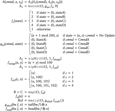
We implement the processes of Figure 9-1 as untimed processes and introduce an additional process Buf. We make our model precise by using the generic process constructors (see Figures 9-2 and 9-3).
Process A is composed of three processes (A1, A2, and A3), and the provided functions define how the processes act in each firing cycle. A1 has a state consisting of two components: a counter counting from 0 through 199, and a state variable remembering the last command. Whenever the counter is 0, a 1, 2, 3, or 4 is emitted depending on the state variable; otherwise a 1 is emitted. This output is used by A3 and function fctrl. Depending on this value, A3, emits 1, 2, 3, or 4 copies of its input to its output. Process A2 merges the input streams x and z4 by means of function fmerge.
A few remarks are in order. Because an untimed model does not allow us to check for the presence or absence of an input value, we model the cmnd input as a stream of values with a specific value, NoUpdate, if nothing changes. This is a rather unnatural way to model control signals with rare events.
The same property of the untimed model causes some trouble for the buffer process. Process A can emit 1, 2, or any number of tokens during one activation. But Buf has to know in advance how many tokens it wants to read. If it tries to read two tokens, but only one is available, it will block and wait for the second. During this time it cannot serve requests from B. We can rectify this by bundling a number of packets into a single token between A and Buf. Buf always reads exactly one token, which may contain 1, 2, 3, or 4 packets. Consequently, in Figure 9-2 function fctrl produces a sequence of values at each invocation, and function fnbuf takes a sequence as second argument.
While this solves our problem, it highlights a fundamental aspect of untimed models as we have defined them. Due to the deterministic behavior with a blocking read it is not obvious how to decouple two processes A and B completely from each other. A truly asynchronous buffer is cumbersome to realize. However, what we can do, and what we want to do in this case, is to fix the relative activation rate of A and B and investigate how the buffer in between behaves. In this respect, untimed models resemble synchronous models. In synchronous models we cannot decouple processes A and B either, but we can observe the buffer in between by exchanging varying amounts of data in each activation cycle. If we want to decouple two processes in a nondeterministic or stochastic way, neither the untimed nor the synchronous model can help us.
The simulation of the model yields quite different results depending on the input sequence. Table 9-1 shows the result of 11 different runs. As input we have used 5000 integers in increasing order. For the first row in the table the input started with 0, 1, 2, ...; for the second row it started with 1, 2, 3, ...; and so on. The last row, marked with a *, the input sequence started with 1, 2, 3, ..., but the function fmerge was not merging the streams x and x4 but just passing on x without modification. The objective for this row was to get a very regular input stream without an irregular distribution of 0s. The second column gives the number of 0s dropped by the buffer; the third column gives the number of 0s inserted by the buffer when it was empty and process B requested data.
Table 9-1. Simulation runs with 5000 samples of consecutive integers.
Sequence start | Dropped 0s | Inserted 0s | 0s% | Buffer length |
|---|---|---|---|---|
0 | 109 | 69 | 2.16 | 14 |
1 | 55 | 11 | 1.09 | 13 |
2 | 45 | 8 | 0.89 | 13 |
3 | 46 | 4 | 0.91 | 9 |
4 | 37 | 2 | 0.73 | 16 |
5 | 75 | 31 | 1.49 | 13 |
6 | 61 | 18 | 1.21 | 12 |
7 | 55 | 12 | 1.09 | 11 |
8 | 41 | 3 | 0.81 | 13 |
9 | 56 | 21 | 1.11 | 15 |
10 | 50 | 11 | 0.99 | 16 |
* | 50 | 6 | 0.99 | 8 |
Table 9-1 shows that the maximum buffer length is very sensibly dependent on the input sequence. If it is a regular stream, like in the last row, the simulation corresponds to our analysis above. But for different inputs we get maximum buffer lengths of anywhere between 8 and 16. Even though the fraction of 0s on the input stream is always 1%, it varies between 0.73% and 2.16% before the buffer. But even when the fraction is similar, like in the last two rows, the maximum buffer length can deviate by a factor of 2.
Besides the great importance of realistic input vectors for any kind of performance simulation, this discussion shows that an untimed model can be used for the performance analysis of parameters unrelated to timing, or rather, to be precise, where we can keep the relative timing fixed in order to understand the relation between other parameters. In this case we examine the impact of control and data input on the maximum buffer size.
The two problems we have encountered when developing the untimed model would be somewhat easier to handle in a synchronous model. The NoUpdate events on the control input, which we had to introduce explicitly, would not be necessary, because we would use the more suitable ⊔ events, which represent absent events, indicating naturally that most of the time no control command is received. The situation of a varying data rate between process A3 and Buf could be handled in two different ways. Either we bundle several packets into one event, as we did in the untimed model, or we reflect the fact that A1 and Buf have to operate at a rate four times higher than other processes. In state δ these two processes have to handle four packets when all other processes have to handle only one. Thus, if we do not assume other buffers, these processes have to operate faster. In the synchronous model we would have four events between A1 and Buf for each event on other streams. Since most of the time only one of these four events would be valid packets, most of the events would be absent (⊔) events. This had the added benefit that we could observe the impact of different relative timing behavior. In an untimed model we can achieve the same, but we have to model absent events explicitly. However, the differences for problems of this kind are not profound, and we record that untimed and synchronous models are equivalent in this respect, but require slightly different modeling techniques.
The timed model confronts us with the need to determine the detailed timing behavior of all involved processes. While this requires more work and is tedious, it gives us more flexibility and generality. We are not restricted to a fixed integer ratio between execution times of processes but can model arbitrary and data-dependent time behavior. Furthermore, we do not need to be concerned with the problem of too tight coupling of the buffer to its adjacent processes. This gained generality, however, comes at the price of less efficient simulation performance and, if a δ-delay-based model is used, a severe obstacle to parallel distributed simulation as discussed in Chapter 5.
We have already started to indicate how different models of computation constrain our ability for analyzing timing behavior that is at the core of performance analysis. To substantiate the discussion, we again use the example of the previous section. We will take the example of Figure 9-2, and replace the definitions of Figure 9-3 with the ones in Figure 9-4.
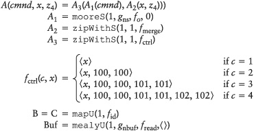
All processes behave identically with the exception of A3, which introduces a delay for the maintenance packets. We have replaced the untimed model with a synchronous one in order to measure the delay of a packet through the network.
Table 9-2 shows the result. The maximum delay of packets through the network is significant. If there is only a single buffer in the system, as in our case, the delay becomes equal to the maximum buffer size. The necessary buffer size has increased compared to Figure 9-1 because B cannot process packets as fast as before and relies on additional buffering. This kind of analysis is natural in a synchronous model because inserting delays that are integer multiples of the basic event execution cycle is straightforward.
Table 9-2. Simulation runs with 5000 samples for Figure 9-4.
Sequence start | Buffer length | Max packet delay |
|---|---|---|
0 | 50 | 50 |
1 | 56 | 56 |
2 | 58 | 58 |
3 | 54 | 54 |
4 | 48 | 48 |
5 | 48 | 48 |
6 | 47 | 47 |
7 | 51 | 51 |
8 | 59 | 59 |
9 | 55 | 55 |
10 | 52 | 52 |
In a product development process the specification is typically the first document, where the extensive discussion of many aspects of the problem leads to a first proposal of a system that will solve the given problem. Hence, the purpose of the specification document is twofold:
P-I. | It is a means to study if the proposed system will indeed be a solution to the posed problem with all its functional and nonfunctional requirements and constraints, that is, to make sure to make the right system. |
P-II. | It defines the functionality and the constraints of the system for the following design and implementation phases. |
From these two purposes we can derive several general requirements for a specification method:
To support the specification process: To write a specification is an iterative process. This process should be supported by a technique that allows the engineer to add, modify, and remove the entities of concern without a large impact on the rest of the specification.
High abstraction: The modeling concepts must be at a high enough abstraction level. The system engineer should not be bothered with modeling details that are not relevant at this stage.
Implementation independent: The system specification should not bias the design and implementation in undesirable ways. System architects must be given as much freedom as possible to evaluate different architecture and implementation alternatives. Products are frequently developed in several versions with different performance and cost characteristics. Ideally the same functional specification should be used for all versions.
Analyzable: The specification should be analyzable in various ways, for example, by simulation, formal verification, performance analysis, and so on.
Base for implementation: The specification should support a systematic technique to derive an efficient implementation. This is in direct conflict with requirements B and C.
In this section we concentrate on the functional part of the specification for the purpose of developing and understanding the system functionality. Item E on the above list, “base for implementation,” will be discussed in the following section on design and synthesis. Some aspects of item D, “analyzable,” have been investigated in the section on performance analysis, and other aspects belong to the realm of formal verification, which is beyond the scope of this book. Hence, here we elaborate on the first three items.
The specification phase comes after the requirements engineering and before the design phase. During requirements engineering all functional and nonfunctional requirements and constraints are formulated. After that, the functional specification describes a system that meets the given constraints. To cut out the space for the functional specification, we introduce two examples and take both from a requirements definition over a functional specification to a design description. The first example is a number sorter, and the second example is a packet multiplexer. After that we discuss the role of the functional specification and what kind of computational model best supports this role.
Figure 9-5 shows the requirements definition of a functional number sorter that converts an indexed array A into another indexed array B that is sorted. The requirements only state the conditions that must hold in order that B is considered to be sorted, but it does not indicate how we could possibly compute B.
Table 9-5. Functional requirements of a number sorter.
sort :: (IntArrayA) ⇒ (IntArrayB)
        Precondition: true
       Postcondition: ∀a: a ∊ A → a ∊ B
                      ∧∀b: b ∊ B → b ∊ A
∧∀i, j ∊ Z, bi, bj ∊ B : i < j → bi ≤ bj |
Figure 9-6 gives us two alternative functional models for sorting an array. The first, sort1, solves the problem recursively by putting sorted subarrays together to form the final sorted array. First comes the sorted array of those elements that are smaller than the first array element (first(A)), and finally the sorted array of those elements that are greater or equal to first(A). The second function, sort2, is also recursively defined and takes all elements that are smallest and puts them in front of the sorted rest of the array. Both functions are equivalent, which can be proved, but they exhibit important differences that affect performance characteristics of possible implementations. One important feature of both function definitions is that potential parallelism is only constrained by data dependences. For example, sort2 does not define if smallest(A) is computed before, in parallel with, or after the rest of the array. In fact, it does not matter for the result in which order the computations are performed. However, the computation is divided into two uneven parts. smallest(A) is inherently simpler to compute than deriving and sorting the rest of the array. This is also obvious from the fact that smallest(A) is even a part of the second computation. Thus, the data dependences will enforce a rather sequential implementation. sort1, on the other hand, has a much higher potential for a parallel implementation because the problem is broken up more evenly. Unless A is not almost sorted, the problems of sorting those elements that are less than first(A) will be as big as sorting those elements that are greater or equal to first(A). Which one of the two functional models is preferable will depend on what kind of implementation will be selected. sort1 is better for a parallel architecture such as an FPGA or a processor array. For a single-processor machine that executes purely sequential programs, sort2 should be preferred because sort1 might be hopelessly inefficient. Figure 9-7 shows a sequential algorithm of function sort2. Several design decisions were taken when refining sort2 into sort2_alg. The amount of parallelism has been fixed, basically by removing the potential parallelism. The representation of the data and how to access it has been determined. Finally, the details of how to compute all functions such as smallest() have been worked out.
The packet multiplexer merges four 150 packets/second streams into one 600 packets/second stream as shown in Figure 9-8. The requirements definition would be mostly concerned with the constraints on the interfaces and the performance of the input and output streams. The functional requirements would state that all packets on the inputs should appear on the output and that the ordering on the input streams should be preserved on the output stream.

A functional model fulfilling these requirements is shown in Figure 9-9. We assume that we have a process constructor zipWith4U, which is a generalization of the previously defined zipWithU and merges four signals into one.
Table 9-9. A functional model of the packet multiplexer as an untimed process.
Mux(s1, s2, s3, s4) = zlpWlth4U(1, 1, 1, 1, f) f(x1, x2, x3, x4) = 〈(x1, x2, x3, x4〉 |
Since the functionality we are asking for is simple, the functional model is short. But a further refined design model could be more involved, as is shown in Figure 9-10. It is based on three simple two-input multiplexers that merge the input stream in two steps. It is refined, although it implements the same functionality, because we made a decision to realize the required function by means of a network of more primitive elements.

Let’s assume that our requirements change and the output does not have a capacity of 600 packets/second but only 450. That means we have to drop one out of four packets and, according to the new requirements, we should avoid buffering packets and drop one packet in each multiplex cycle. If there is an idle packet, we should drop it; otherwise it does not matter which one we lose. A new functional description, which meets the new requirements, is shown in Figure 9-11. The function f outputs only three of the four input packets, and it drops the packet from stream s4 if none of the other packets is idle. When we propagate the modification down to the design model, we have several possibilities, depending on where we insert the new functionality. It could become part of modified Mux-2 blocks, or it could be realized by a separate new block before the output. We could also distribute it and filter out all idle packets at the inputs, and either insert idle packets or filter out a packet from stream s4 before the output. The solution we have chosen, as shown in Figure 9-12, inserts two new blocks, filter_idle, which communicate with each other to filter out the right packet.

The borderlines between requirements definition, functional specification, and design are blurred because in principle it is a gradual refinement process. Design decisions are added step by step, and the models are steadily enriched with details, which eventually leads hopefully to a working system that meets the requirements. Hence, to some degree it is arbitrary which model is called the requirements definition, functional specification, or design description, and in which phase which decisions are taken. On the other hand, organizing the design process into distinct phases and using different modeling concepts for different tasks is unavoidable.
In the number sorter example, we have made several design decisions on the way from the requirements definition to a sequential program. We have not made all the decisions at once but rather in two steps. In the first step, which ended with a functional model (Figure 9-6), we broke the problem up into smaller subproblems and defined how to generate the solution from the subsolutions. The way we do this constrains the potential parallelism. In addition, the breaking the problem up into subproblems will also constrain the type of communication necessary between the computations solving the subproblems. This may have severe consequences for performance if a distributed implementation is selected.
While these observations may be self-evident, for the number sorter it is less obvious that we need a functional model at all. It might be preferable to develop a detailed implementation directly from the requirements definition because the best choice on how to break up the problem only becomes apparent when we work on the detailed implementation with a concrete architecture in mind. Neither sort1 nor sort2 is clearly better than the other; it depends on the concrete route to implementation.
Although this is correct and might render a functional model for simple examples useless, the situation is more difficult for the development of larger systems. First, with the introduction of a functional model the design decisions between requirements definition and implementation model are separated into two groups. Since the number of decisions may be very large and overwhelming, to group them in a systematic way will lead to better decisions. This is true in particular if certain issues are better analyzed and explored with one kind of model than with another. One issue that is better investigated with a functional model, as we have exposed with the number sorter example, is the potential parallelism and, as a consequence, the constraints on dataflow and communication between the computations of subproblems. However, this does not rule out taking into account the different architectures for the implementation. On the contrary, in order to analyze sensibly different functional alternatives, we must do this with respect to the characteristics of alternative architectures and implementations.
Another issue where a functional model may support a systematic exploration is revealed by the second example, the packet multiplexer. The functional design phase must explore the function space. Which functions should be included or excluded? Can a given set of functions meet user needs and requirements? These user needs and requirements are sometimes only vaguely specified and may require extensive analysis and simulation. For instance, the convenience of a user interface can often only be assessed when simulated and tried by a user. The impact of adding or deleting a function on other parts of the system is sometimes not obvious. For instance, the change of functionality in the packet multiplexer example, which means that up to 100% of the packets in stream s4 are lost, may have undesirable consequences for the rest of the telecommunication network. It might be worthwhile to evaluate the impact of this change by an extensive simulation. A functional model can greatly facilitate these explorations provided we can quickly modify, add, and remove functions. In contrast, the consecutive design phase is much more concerned with mapping a functionality onto a network of available or synthesizable components, evaluating alternative topologies of this network, and, in general, finding efficient and feasible implementations for a fixed functionality. If these two distinct objectives are unconsciously mixed up, it may lead to an inefficient and unsystematic exploration of alternatives. In the case of the packet multiplexer it is unnecessary to investigate with great effort the best place to insert the new filter functionality or to modify the existing Mux-2 blocks if a functional system simulation reveals that the new functionality has undesirable consequences and must be modified or withdrawn.
From these considerations we can draw some conclusions on how best to support purpose P-I of a functional specification. In order to efficiently write and modify a specification document, we should avoid all irrelevant details. Unfortunately, what is relevant and what is not relevant is not constant and depends on the context.
Time: Frequently timing is not an issue when we explore functionality, and consequently information on timing should be absent. But for almost every complex system, not just real-time systems, there comes a point when timing and performance must be considered as part of the functional exploration. As we have seen in the previous section on performance analyses, most analysis of nonfunctional properties will involve considerations about time. In light of this argument, we may reason that a synchronous model may be best because, on the one hand, it makes default assumptions about time that alleviate the user from dealing with it when not necessary. On the other hand, it allows us to make assumptions about the timing behavior of processes that can be used both as part of the functional simulation and can serve as timing constraints for the consecutive design phases.
Concurrency: As we have seen in the number sorter example, the functional specification phase breaks up the problem into subproblems and explores potential parallelism. The models of computation that we have reviewed are all models with explicit concurrency. But for functional exploration, the boundaries between concurrent processes should not be too distinct, and functionality should be easily moved from one process to another. Thus, either we should avoid explicit concurrency altogether, only using models of implicit concurrency such as a purely functional model, or we should use the same modeling concepts inside processes as between processes. For instance, if we have a hierarchical untimed process network without a distinction between a coordination and a host language, the process boundaries can be easily moved up and down the hierarchy (Skillicorn and Talia 1998a).
Primitive functions: The primitive elements available are as important as the computational model and are often application specific. For instance, various filters and vector transformation functions are required for signal-processing applications, while control-dominated applications need control constructs, finite state machines, exceptions, and similar features. Obviously, the availability of an appropriate library makes the modeling and design process significantly more efficient.
Avoiding details: The kind and the amount of details in a model is determined by three factors: (a) the abstraction levels in the four domains of computation, communication, time, and data; (b) the primitive functions and components available; (c) the modeling style of the designer. Given (a) and (b), the designer still has significant choice in modeling and how to use languages and libraries.
With respect to purpose P-II we refer to the following discussion of design and synthesis.
Manual design and automatic synthesis are at the core of the engineering task of creating an electronic system. After having determined the functionality of the system, we must create a physical device that implements the functionality. Essentially, this is a decision-making process that gradually accumulates a huge amount of design information and details. It can be viewed as going from a high abstraction level, which captures the basic functionality and contains relative few details, to ever lower abstraction levels with ever more details. This is quite a long way, stretching from a system functionality model to a hardware and software implementation. The hardware implementation is a description of the geometry of the masks that are direct inputs to the manufacturing process in a semiconductor foundry. For software it is sequence of instructions that control the execution of a processor. A huge number of different design decisions have to be taken along this way, for instance, the selection of the target technology, the selection of the components and libraries, the architecture, the memory system, the hardware/software distribution, and so on.
In general we can observe that we use a combination of two techniques:
Top-down: synthesis and mapping
Bottom-up: use of components and libraries
If our problem is such that we can find a component in our library that solves the problem directly, we skip the top-down phase, select the right component, and we are done. In this case, although we might be very happy, we would hardly call our activity a system design task. On the other hand, we always have a set of primitive components, from which we must select and assemble to get a device solving our problem. These components may be simple and tiny, such as transistors or instructions for a processor, or they may be large and complex, such as processors, boards, databases, or word processors. Curiously, the synthesis and mapping phase tends to be rather shallow. During the last 30 years the complexity of the “primitive” components has tightly followed the complexity of the functionality of electronic systems. While the “system functionality” developed from combinatorial functions to sequential datapaths and complex controllers to a collection of communicating tasks, the “primitive library components” evolved from transistors to complex logic gates to specialized functional blocks and general processor cores. Attempts to cross several abstraction levels by means of automatic synthesis, such as high-level synthesis tools, have in general not been very successful and have typically been superseded by simpler synthesis tools that map the functionality onto more complex components. The latest wave of this kind has established processor cores as “primitive components.”
In the following we discuss in general terms a number of system design problems in order to understand what kind of information has to be captured by different models and how one kind of model is transformed into another. This will allow us to assess how adequate the models of computations are to support these activities.
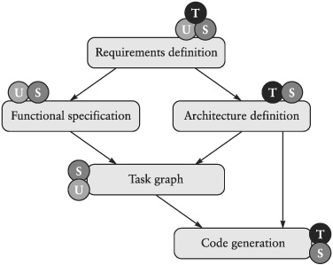
We use a simple design flow as illustrated in Figure 9-13 to discuss the major design tasks and their relation. This flow is simplified and idealistic in that it does not show feedback loops, while in reality we always have iterations and many dependences. For instance, some requirements may depend on specific assumptions of the architecture, and the development of the task graph may influence all earlier phases. But this simple flow suffices here to identify all important design and synthesis activities and to put them in the proper context.

Figure 9-13. System design flow from requirements engineering to code generation of hardware and software.
In addition to the functional specification, the architecture has to be defined. The architecture is not derived from the functional specification but is the second major independent input to the consecutive design and implementation phases. The architecture cannot be derived from a given functionality for two reasons. First, the number of possible architectures (i.e., the design space) is simply too large. There is no way that a tool or a human designer can systematically consider and assess a significant part of all potentially feasible architectures. But this is not really necessary either because we have experience and a good understanding of which kinds of architectures are efficient and cost effective for a given application. Hence, we only need to assess a few variants of these proven architectures. Second, designers typically face constraints about the architectures they can use. These constraints may spring up from a number of sources. Perhaps we must design only a subpart of a system that has to fit physically and logically to the rest of the system. Or maybe our company has special deals with a particular supplier of a processor, a board, or an operating system, forcing us to use these elements rather than something else. Another source of constraints is that we have to design not just one product but a family of products, and we have to consider all of them at the same time. Consequently, the architecture is always defined almost independently from the definition of the functionality, and it is an important input to the following steps of task graph design and code generation. To define an architecture basically means to select a set of components and a structure to connect them.
The selection of the components and the design of the topology can be a very intricate problem. First, component selection is often hierarchical both for software and hardware components. We have to choose a library from a particular vendor or for a specific technology. From the libraries we select the components for our design. The alternative libraries are usually not equivalent or directly comparable. Certain components may be faster in one library than in another; others may be slower. Some components may not be available in a library, forcing us to find alternative solutions based on a combination of other components. Second, the selection of individual components is not independent from the selection of other components. The choice of one particular microprocessor core determines or constrains the kind of bus we can use, which in turn constrains the selection of other components. The processor also imposes constraints on the memory system and caches, which may have far-reaching consequences for system performance and software code size, which in turn may affect the task partitioning, software component selection, and scheduling policy.
Not only are components organized hierarchically into libraries, but also the assembly of components are organized in a hierarchy of architectures. We may have a system architecture, a board architecture, and a chip architecture. The software may also be organized in a hierarchical architecture comprising several layers.
These observations illustrate that the selection of components and the design of architectures are indeed intricate tasks. Many alternatives must be considered, assessed, and compared. This demands that we are able to model the components and their composition with respect to functional and nonfunctional features.
The system functionality must be partitioned into tasks, which in turn must be mapped onto the network of allocated components. Again, this involves many delicate, interdependent decisions. Some of the important activities are the partitioning into tasks and the mapping of tasks onto resources such as processors, micro controllers, DSPs, FPGAs, custom hardware, and so on. For tasks mapped to software, the scheduling policy must be determined. Scheduling can be static and decided during design time, or dynamic during run time. In the latter case a run-time scheduler must be included. Each task must then be implemented, which means the generation of executable code for software and a layout description for hardware. The design and synthesis of interfaces and communication code between tasks and components is one of the most troublesome and error-prone activities.
This brief review of design problems allows us to identify some requirements on modeling. One obvious observation is that the assessment of nonfunctional properties is an integral task of most design activities. Unfortunately, nonfunctional properties, with the notable exception of time, are not an integral part of most modeling techniques and modeling languages. Since our theme is the analysis of computational models, we can only acknowledge this situation and restrict further discussion to issues of functionality and time.
To model components and networks of components realistically, we should employ a timed model because it is the only metamodel that can capture the timing behavior with arbitrary precision. This may not always be necessary; in fact in many cases it is not. When we only deal with the functionality, the delay of individual components is irrelevant. In other cases we are content with a more abstract notion of time corresponding to a synchronous model. For instance, in hardware design the very popular synchronous logic partitions a design into combinatorial blocks separated by latches or registers, as illustrated in Figure 9-14. The edge-triggered registers at the inputs and outputs of the combinatorial block are controlled by the rising edge of a clock signal. Thus, when the clock signal rises, the inputs a, b, c, and d to the combinatorial block change and the gates react by changing their respective outputs as appropriate. When the clock signal rises the next time, the outputs y and z are stored in the output registers and are thus available for the next combinatorial block.

This allows us to separate timing issues from functionality issues; in the first step we assume that all combinatorial blocks are fast enough to deliver a result within a clock period, and in the second step we verify that this assumption is in fact correct. Thus, the first step does not require a timed model but only an untimed or a synchronous model. It is indeed an order of magnitude more efficient to simulate such designs in a synchronous timing model as the cycle-true simulators have proven. Only the second step requires a timed model, but even there we can separate timing from functionality by means of a static timing analysis. For the example in Figure 9-14 the static timing analysis would calculate the longest path, which is from input a to output y, and takes 8 ns. Thus, when any of the inputs change, all outputs would be available after 8 ns and the clock cycle needs to be no longer than 8 ns.
Consequently we could describe the functionality of a component based on an untimed model that just represents the input-output behavior, and store the timing information as a separate annotation. But even though the actual use of accurate timing information is limited, using the timed model for component modeling is still recommended for two reasons. First, almost always comes a situation where it is mandatory, for instance, when the behavior depends on the precise timing or vice versa, and this is relevant. Static timing analysis can only reveal the worst-case delay. However, when this worst case can never happen because the input vector to a combinatorial block is inherently restricted by another block, static timing analysis would be too conservative. For instance, assume that in the example of Figure 9-14 the inputs are constrained such that a is always equal to b. The AND gate that connects NOT a and b would always have an output of 0 and would never change, no matter what the inputs were, if we ignore glitches. The longest path would be 5 ns from d to y. Such situations cannot be detected by static analysis or functional simulation alone. Only when we analyze the functional behavior and the timing of the components together can we detect this. The second reason why we prefer a timed model for modeling components and structure is that timing information can be easily ignored when components are included in a simulation based on another computational model, as has been shown with functional and cycle true simulations.
Another main concern for modeling is the transformation of functionality during the design process. System functions are partitioned into tasks, communication between tasks is refined from high-level to low-level protocols, parallel computations are serialized and vice versa, functions are transformed until they can be mapped onto a given network of primitive components, and so on and so on. If all this is done manually, we do not have much to worry about, at least not for the design process itself. We must still worry about validation. For an automatic synthesis process the situation is more delicate because all the transformations and refinements must be correct. While it is possible—and even popular—to hardwire rules into the synthesis tool, this process can be supported more systematically and in a more general way by providing large classes of equivalences. Whenever we have a case of semantic equivalence a tool can use this to transform a given design into a more optimal implementation. For instance, for a function over integers f1(x) = h(x) + g(x), the commutative law tells us that this is equivalent to f2(x) = g(x) + h(x). A synthesis tool could then transform f1 into f2 if the hardware structure is such that the latter represents a more efficient implementation. However, if this is not guaranteed by the semantics of the language, such a transformation is not possible and the exploration space of the synthesis tool is significantly restricted. For instance in C this particular equivalence is not guaranteed because g and h may have side effects that may change the result if they are evaluated in a different order.
The essential difference of the three main computational models that we introduced in Chapters 3 through 5 is the representation of time. This feature alone weighs heavily with respect to their suitability for design tasks and development phases.
The timed model has the significant drawback that precise delay information cannot be synthesized. To specify a specific delay model for a piece of computation may be useful for simulation and may be appropriate for an existing component, but it hopelessly overspecifies the computation for synthesis. Assume a multiplication is defined to take 5 ns. Shall the synthesis tool try to get as close to this figure as possible? What deviation is acceptable? Or should it be interpreted as “max 5 ns”? Different tools will give different answers to these questions. Synthesis for different target technologies will yield very different results, and none of them will match the simulation of the DE model. The situation becomes even worse when a δ-delay-based model is used. As we discussed in Chapter 5 the δ-delay model elegantly serves the problem of nondeterminism for simulation, but it requires a mechanism for globally ordering the events. Essentially, a synthesis system had to synthesize a similar mechanism together with the target design, which is an unacceptable overhead.
These problems notwithstanding, synthesis systems for both hardware and software have been developed for languages based on timed models. VHDL- and Verilog-based tools are the most popular and successful examples. They have avoided these problems by ignoring the discrete event model and interpreting the specification according to a clocked synchronous model. Specific coding rules and assumptions allow the tool to identify a clock signal and infer latches or registers separating the combinatorial blocks. The drawbacks of this approach are that one has to follow special coding guidelines for synthesis, that specification and implementation may behave differently, and in general that the semantics of the language is complicated by distinguishing between a simulation and a synthesis semantics. The success of this approach illustrates the suitability of the clocked synchronous model for synthesis but underscores that the untimed model is not synthesizable. Apparently, this does not preclude efficient synthesis for languages based on the untimed model, even though it comes at a cost.
The synchronous models represent a sensible compromise between untimed and fully timed models. Most of the timing details can be ignored, but we can still use an abstract time unit, the evaluation or clock cycle, to reason about the timing behavior. Therefore it often has a natural place as an intermediate model in the design process. Lower-level synthesis may start from a synchronous model. Logic and RTL synthesis for hardware design and the compilation of synchronous languages for embedded software are prominent examples. The result of certain synthesis steps may also be represented as a synchronous description such as scheduling and behavioral synthesis.
It is debatable if a synchronous model is an appropriate starting point for higher-level synthesis and design activities. It fairly strictly defines that activities occurring in the same evaluation cycle but in independent processes are simultaneous. This imposes a rather strong coupling between unrelated processes and may restrict early design and synthesis activities too much.
As we saw in Section 3.15, the dataflow process networks and their variants have nice mathematical features that facilitate certain synthesis tasks. The tedious scheduling problem for software implementations is well understood and efficiently solvable for synchronous and boolean dataflow graphs. The same can be said for determining the right buffer sizes between processes, which is a necessary and critical task for hardware, software, and mixed implementations. How well the individual processes can be compiled to hardware or software depends on the language used to describe them. The dataflow process model does not restrict the choice of these languages and is therefore not responsible for their support. For what it is responsible—the communication between processes and their relative timing—it provides excellent support due to a carefully devised mathematical model.
Figure 9-15 summarizes this discussion and indicates in which design phases the different MoCs are most suitable.
Many good books describe various performance-modeling techniques in detail. Examples are Cassandras (1993) and Severance (2001).
There are also several texts that discuss the subject of functional system specification. However, the presentation of this subject varies considerably since no standard point of view has been established yet. Gajski and co-workers have taken up an extensive general discussion several times while introducing a concrete language and methodology, SpecChart (Gajski et al. 1994) and SpecC (Gajski et al. 2000). Both books also discuss the design and synthesis aspects of models.
A more formal approach is described by van der Putten and Voeten (1997). Another very formal approach, based on abstract algebra, is given by Ehrig and Mahr (1985).
There are a large number of methodology-oriented books on specification and design. A classic book on structured analysis and specification is DeMarco (1978). Good introductions to object-oriented analysis and specification are Selic et al. (1994), Yourdon (1994), and Coad and Yourdon (1991).
9.1 | Given is a switch and a number of n resources, all directly connected to the switch, as shown in Figure 9-16. Every resource sends packets to another resource with a probability of pn. The destination resource is selected randomly with a uniform distribution; that is, the probability to select a particular resource is The switch operates with a cycle time cs = ρcr, ρ ≥ 1, where cr is the cycle time of the resources. Thus, the switch can send and receive ρ packets, while a resource can send and receive only 1 packet. The switch has a central queue with length q. If a new packet arrives when the buffer is full, the new packet is discarded. What is the probability of losing a packet due to buffer overflow? Make a simulation model with the following parameters:
Simulate with 1000, 10,000, and 100,000 cycles to see which probability is approximated. |
9.2 | Develop and model the data link protocol layer of the architecture of Exercise 9.1. The switch is connected to each resource node by a 32-bit bus and a few control lines. You may introduce and use a reasonable number of control lines such as “REQUEST,” “ACKNOWLEDGE,” “DATA VALID,” and so on. The switch and the resource run with different clocks at different speeds and with different phases. No assumptions can be made about the relationship of the clocks. Both the switch and the resource can initiate a data transfer. Develop a protocol to exchange data between the switch and the resource, based on 32-bit words. The package size is fixed with 16 words. The protocol should be reliable; thus the protocol is not allowed to lose packets. Optimize the latency and the throughput for both very low and very high data rates. You may use either the synchronous or the untimed MoC. |
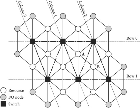
9.3 | Given is a honeycomb network of resources and switches (Figure 9-17) with s switches, r resources, o of which are I/O resources.r (1) = 6, r (s) = 3s +4, s > 1; o(1) = 6, o (s) =s + 6, s > 1. The switches are organized in rows and columns as shown in Figure 9-17. In this way each switch gets a unique address, which consists of the row and the column number <row#,col#>. A resource gets the coordinates of the switch to which it is connected plus a third number, which determines its position in the hexagon of the switch. This number, called “wind”, is between 0 and 5 and is defined as follows: 0 = N, 1 = NE, 2 = SE, 3 = S, 4 = SW, 5 = NW. To avoid multiple addresses for the same resource, we define that only row 0 has wind = 0,1, and 5; all other rows have only the bottom half of the wind coordinates. Similarly, only column 0 has wind = 4 and 5, all others have only the right part of the wind coordinates. In this way all resources have a unique address. For example, resource A in Figure 9-17 has the coordinates <row = 0, col = 1, wind = 2>, while B has <row = 0, col = 2, wind = 3>. Every resource sends packets to another resource with a probability of pr. The destination resource is selected randomly with a uniform distribution; that is, the probability to select a particular resource is The routing in the network follows some rules. If source and destination are directly connected, they communicate directly; otherwise the source sends the packet to the switch to which it is associated, then the packet is handed from switch to switch until it reaches the switch to which the destination is associated. The routing tables in the switches are set up such that a packet is first transferred to the destination row and then to the destination column. The switches operate with a cycle time cs = ρcr, ρ ≥ 1; that is, a switch can send and receive ρ packets, while a resource can send and receive only 1 packet. The switches have central queues with length q. If a new packet arrives when the buffer is full, the new packet is discarded. What is the probability of losing a packet due to buffer overflow? Make a simulation model with the following parameters:
Simulate with 1000, 10,000, and 100,000 cycles to see which probability is approximated. |
9.4 | Repeat Exercise 9.3 with an additional locality assumption. The probability of selecting a particular destination resource is a function of the distance dr to this resource. The probability that a resource sends a packet to another resource at distance d is where D is the maximum possible distance and Hence, A(D) is a normalization factor that guarantees that the sum of the probabilities is 1. The probability of selecting a particular resource from resources with the same distance from the sending node is uniformly distributed. |
9.5 | Develop and model the network layer protocol of the NOC architecture of Exercise 9.3 for both the switches and the resources. Use the data link protocol for the communication between individual switches and resources. Provide a reliable service for the next higher layer without acknowledgment; that is, that an application uses the network layer by calling it with a packet and the destination address. Then the application can be assured that the packet will receive the destination, and it does not expect any acknowledgment. |