
Frequency-Domain Based DFIG Wind Energy Systems Modeling
Abstract
This chapter presents frequency-domain based modeling techniques for doubly fed induction generator (DFIG) wind energy systems. Two types of frequency-domain modeling approaches are presented. The first type is impedance model. Impedance represents the ratio of the terminal voltage and the through current of a device in frequency domain. Using impedance models, a circuit analysis problem is converted to a feedback control system problem. Resonances can be identified using tools for control systems, for example, Nyquist stability criteria and Bode plots. The positive-sequence impedance model for a Type-3 series compensated wind energy system is developed. Subsynchronous resonance (SSR) is then identified. Negative-sequence impedance model is also developed to examine the effect of unbalance in stator voltage on SSR. The second type of frequency-domain model is torque/speed transfer function, which is popularly used for torsional interaction investigation. Torque/speed transfer function including DFIG’s effect is derived to examine torsional interactions. Further, effect of unbalance in stator voltage on torsional interactions is examined.
In this chapter, DFIG’s frequency-domain models at different reference frames (phase domain, dq reference frame) will be derived and explained. Then three examples on using the frequency-domain models for SSR analysis and torsional interaction analysis will be presented.
The chapter is organized in four sections. In Section 6.1, introduction of impedance model and its application in stability and resonance detection will be given. In Section 6.2, impedance models of DFIG in various reference frames, e.g., abc and dq, will be derived. In Section 6.3, negative-sequence impedance model is derived. In Section 6.4, inclusion of DFIG impedance model into a torque-speed transfer function will be presented. Section 6.5 presents three examples. The first example considers only balanced operating conditions and presents SSR detection using abc-domain impedance models. The second example considers unbalanced conditions and explains the impact of negative-sequence stator voltage on SSR using negative sequence impedance models. The third example uses torque-speed transfer function to explain DFIG’s influence on torsional interactions.
6.1 Introduction of Impedance Model and Its Application in Stability and Resonance Detection
Impedance-based models and Nyquist stability criterion provide insights on electric resonances. Such methods have been widely adopted in power electronics and system interaction studies [1, 2]. More recently, interactions between a grid-connected voltage source converter’s current controllers and large network inductances are addressed in [3] using impedance models.
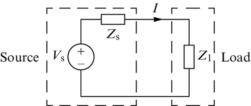
Impedance-based analysis has been applied in power electronic converter analysis in [1, 2]. For a system with a source impedance and load impedance as shown in Fig. 6.1, the current can be calculated as

Assuming that the voltage source is stable and the load is stable when powered from an ideal voltage source, then for the system to be stable, the denominator 1 + Zs(s)/Zl(s) should have all zeros in the open left-half plane (LHP). Based on Nyquist stability criterion, if and only if the number of counter-clockwise encirclement around (−1,0) of Zs/Zl is equal to the number of the right-half plane (RHP) poles of Zs/Zl , the system will be stable. In cases when Zs/Zl has no RHP poles, the Nyquist map of Zs/Zl should not encircle (−1,0).
Instability happens when Zs/Zl encircles (−1,0). In addition, Bode plots can be used to analyze resonance stability. Bode plots of the source impedance and the load impedance can be placed together to identify the phase margin when the magnitudes of the two impedances are the same. This technique has been employed by Sun [2].
Impedance-based modeling technique converts a circuit analysis problem to a feedback control problem shown in Fig. 6.2. Analysis tools for linear control systems, e.g., Nyquist stability criteria, Bode plots, can then be deployed for stability and resonance analysis.

6.2 Impedance Models of DFIG in Various Reference Frames
A study system consisting of a Type-3 DFIG-based wind generator with partial back-to-back voltage source converters and a series-compensated network is again shown in Fig. 6.3. A DFIG-based wind farm (100 MW from aggregation of 2 MW units) is connected to a 161 kV series-compensated line. The collective behavior of a group of wind turbines is represented by an equivalent lumped machine. Xtg represents the combination of the inductive filter at the GSC and a transformer.

The impedance models for the series-compensated network and the DFIG system will be developed in this section. For a three-phase system, impedance model can be expressed in either space vector or dq synchronous reference frame. A space vector voltage relates to the instantaneous three-phase voltages as follows:
where ![]() .
.
6.2.1 RLC Circuit Impedance Model
Assume that the series-compensated network has no mutual inductance and the three phases are symmetrical. For such a three-phase RLC circuit, the impedance model observed in space vector can be expressed as
6.2.2 Induction Machine Impedance Model
To find out the impedance model of a DFIG, we start to find out the relationship between the stator voltage and the stator current. Essentially, it is just to find the equivalent Thevenin impedance and the equivalent Thevenin voltage for the induction machine circuit in space vector (shown in Fig. 6.4).

A few steps can lead us to the stator voltage expression in terms of stator current and rotor voltage solely.
Observe the dynamic model in space vector:
We will first find the expression of ![]() by
by ![]() and
and ![]() from the rotor voltage and rotor flux relationship, shown in (6.9). Then in the stator voltage and stator flux relationship, the rotor current will be replaced by the following expression:
from the rotor voltage and rotor flux relationship, shown in (6.9). Then in the stator voltage and stator flux relationship, the rotor current will be replaced by the following expression:
The stator voltage can be expressed as follows:

Note a space vector based on the stationary frame is related with a complex vector based on the qd reference frame (rotating speed is ω) is as follows:
In the frequency domain, their relation becomes
Therefore, in complex vector, the stator voltage is expressed by replacing s in (6.10) with s + jω.
If Lm is very large compared to the other parameters, then the above equation can be simplified as
The above derivation corroborates with the following analysis on slip. Slip is related to the rotating speed ωm and the stator frequency ω. For the per-phase induction machine circuit shown in Fig. 6.5, the rotating speed can be assumed to be constant since mechanical dynamics is much slower than the electric dynamics. Slip can be expressed as 1 − ωm/ω. In Laplace domain, slip can be expressed as

Hence, the impedance of the DFIG seen from its terminal can be represented by
The above derivation also proves that the impedance model can be developed using the per-phase circuit of a DFIG. The simplified DFIG impedance in (6.15) ignoring RSC and GSC is adopted in [4].
6.2.3 Converter Impedance Model
Cascaded control loops are used in converters in wind generators. The control loops consist of the fast inner current control loops and the slow outer power/voltage control loops. The current control loops usually have bandwidths at or greater than 100 Hz while the outer control loops usually have bandwidths less than several Hz. For SSR studies, the dynamics of interest are much faster than the outer control loops. Thus, the outer control is considered to be constant and will not be included in the impedance model.
For the vector current control scheme in Fig. 6.6, the qd-axis voltage and current relationship is
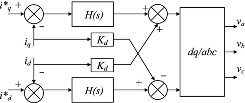
This leads to the expression in complex vector
To view the current controlled converter from space vector, then
For the GSC at positive sequence scenarios, it can be represented by a voltage source ![]() behind an impedance ZGSC, where ZGSC = Hg(s − jω) − jKdg.
behind an impedance ZGSC, where ZGSC = Hg(s − jω) − jKdg.
For the RSC at positive sequence scenarios, it can also be represented by a voltage source ![]() behind an impedance ZRSC where ZRSC = Hr(s − jω) − jKdr.
behind an impedance ZRSC where ZRSC = Hr(s − jω) − jKdr.
6.2.4 Overall Circuit
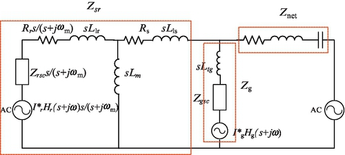
The overall circuit is now shown in Fig. 6.7. The circuit consists of two impedances: the network impedance Znet and the DFIG impedance ZDFIG.

When the gains of the RSC controller KpKi and the feed forward gain Kdr are assumed to be zero, the RSC output voltage will no longer vary even there exists error in measured currents and the reference currents. The RSC can be viewed as a constant voltage source in this case.
6.2.5 Comparison of Zsr and Zg
The DFIG impedance consists of two parallel components: the stator and rotor (including RSC) Zsr and the GSC branch including the GSC and the filter: Zg = ZGSC + sLtg. Bode plots of the RLC network impedances, Zsr and Zg at 95% rotating speed (or 57 Hz) and 50% compensation level are plotted in Fig. 6.8. Zsr is plotted for two scenarios: with and without current PI controllers. When the PI controller gain is not zero, Zsr has two peaks: one at 57 Hz and the other at 60 Hz. When the gain is zero, Zsr however has just one peak at 57 Hz. For Zg, the resonant frequency is 60 Hz. The network impedance has a resonant frequency at 37.5 Hz, which correspond to the 50% compensation level. The network resonant frequency is expressed as:
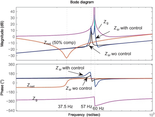
where Xc is the series capacitor reactance, Xline and XT are the line reactance and the transformer reactance.
It is observed that at the interested SSR frequency region (<37.5 Hz), the magnitude of Zg is much larger than Zsr. Therefore, Zsr is dominant. For the SSR analysis, the impact of Zg will be ignored (ZDFIG = Zsr).
6.3 Negative-Sequence DFIG Impedance Model
When the system has both positive and negative sequence components, and let ![]() and
and ![]() be the positive and negative sequence components in
be the positive and negative sequence components in ![]() where
where ![]() is the dynamic phasor of the phase a voltage at the fundamental frequency.
is the dynamic phasor of the phase a voltage at the fundamental frequency.
The phasors are related to the instantaneous variables as follows:

where a =ej2π/3.
The space vector of the terminal voltage is defined as
The space vector can also be expressed in terms of positive and negative sequence phasors
In Laplace domain, the voltage and current space vectors can be written as

When there is only positive sequence or negative sequence, then the impedance observed based on space vectors should have the following relationship with the impedance observed based on the complex vectors or dynamic phasor.

Since the expression of ![]() and
and ![]() are the same, it can be found that
are the same, it can be found that
6.3.1 RLC Circuit
For a three-phase RLC circuit, the impedance model observed in space vector can be expressed as:
The above expression also fits (6.26). Since there is no imaginary part for the positive sequence expression, the negative sequence and the positive sequence expressions are the same.
6.3.2 Induction Machine Impedance Model
We already have the relationship between the stator voltage and stator current, rotor voltage in dq reference frame:
Therefore, a Thevenin equivalent circuit for the induction machine can be developed. Notice that the impedance Z(s) is based on the dq-reference frame. Since the RLC circuit is expressed in the abc reference frame, it will be convenient that there is also an impedance model based on the abc reference frame.
In space vector the stator voltage can be expressed as follows by replacing s by s − jω for positive sequence.
Positive sequence:
Therefore, the positive sequence impedance model is
The negative sequence impedance model is

6.3.3 Converter Impedance Model
Cascaded control loops are used in converters in wind generators. The control loops consist of the fast inner current control loops and the slow outer power/voltage control loops. The current control loops usually have bandwidths at or greater than 100 Hz while the outer control loops usually have bandwidths less than several Hz. For SSR studies, the study dynamics is considered faster than the outer control loops. Thus, the outer control is considered to be constant and will not be included in the impedance model.
For the vector current control scheme in Fig. 6.6, the qd-axis voltage and current relationship is
This leads to the expression in complex vector:
To view the current controlled converter from space vector, then:

For the GSC converter at positive sequence scenarios, it can be represented by a voltage source ![]() behind an impedance ZGSC where ZGSC = Hg(s − jω) − jKdg. At negative sequence scenarios, the GSC converter can be represented by a voltage source
behind an impedance ZGSC where ZGSC = Hg(s − jω) − jKdg. At negative sequence scenarios, the GSC converter can be represented by a voltage source ![]() behind an impedance ZGSC where ZGSC = Hg(s + jω) + jKdg.
behind an impedance ZGSC where ZGSC = Hg(s + jω) + jKdg.
For the RSC converter at positive sequence scenarios, it can also be represented by a voltage source ![]() behind an impedance ZRSC where ZRSC = Hr(s − jω) − jKdr. The negative sequence impedance of the RSC is the conjugate of ZRSC and can be expressed as Hr(s + jω) + jKdr.
behind an impedance ZRSC where ZRSC = Hr(s − jω) − jKdr. The negative sequence impedance of the RSC is the conjugate of ZRSC and can be expressed as Hr(s + jω) + jKdr.
6.3.4 Overall Circuit
The overall circuit for negative sequence is now shown in Fig. 6.9.
6.4 Inclusion of DFIG into Torque-Speed Transfer Functions
To investigate the impact of negative sequence components on torsional interaction, transfer function of the electromagnetic torque (Te) versus the rotating speed (ωm) is developed in this section. The interactions of torque and speed relationship is represented in Fig. 6.10 [5], where Ge(s) represents the relationship of Te versus ωm through electrical system and Gm(s) represents the relationship of ωm and Te through mechanical system. Note the positive feedback is due to the motor convention used in this chapter. When operated as a generator, Te is a negative number.

Therefore the electromagnetic torque and speed transfer function is:
6.4.1 Mechanical System
A two-mass system [6, 7] is used to the represent torsional dynamics given by

where ωt and ωr are the turbine and generator rotor speed, respectively; Pm and Pe are the mechanical power of the turbine and the electrical power of the generator, respectively; T12 is an internal torque of the model; Ht and Hg are the inertia constants of the turbine and the generator, respectively; Dt and Dg are the mechanical damping coefficients of the turbine and the generator, respectively; Dtg is the damping coefficient of the flexible coupling (shaft) between the two masses; Ktg is the shaft stiffness.
From the two-mass mechanical system model, the transfer functions ![]() and
and ![]() can be found.
can be found.
6.4.2 Electrical System
Torque-speed transfer function has been used in [8] to examine torsional interactions. The voltage and current relationship for an induction machine (2.53) in the dq reference frame are linearized. These equations are presented again here.

where ωb = 377 rad/s and the rest variables are in per unit.
The resulting linearized differential equations are as follows:
where isr = [iqs,ids,iqr,idr]T, vs = [vqs,vds]T and vr = [vqr,vdr]T,
where ![]() ,
,

In Laplace domain, the above equation becomes:
Consider the current control loops in the RSC, the RSC voltage can be expressed as:
If we assume that the converter outer control loops can be ignored, then the reference signal ![]() are constants and its deviation is zero.
are constants and its deviation is zero.
Substituting Δvr′ in (6.43) by (6.44) leads to:
It is obvious to find the expression of Δis in terms of the rotating speed and the stator voltage:
The expressions can be developed for both positive and negative sequences. For positive sequence, the DQ reference frame (dq+) is rotating counter clockwise at nominal frequency ω. While for negative sequence, the DQ reference frame is rotating clockwise at the nominal frequency ω. The major differences in expressions are A1 and ZRSC. For positive sequence, since the vector control is based on the same reference frame, ![]() . However, for negative sequence, since the vector control is based on dq+ while the model is based on dq−, the impedance of the RSC should be converted to qd−. Hence
. However, for negative sequence, since the vector control is based on dq+ while the model is based on dq−, the impedance of the RSC should be converted to qd−. Hence ![]() .
.
where the superscripts “+” and “−” represent the dq + and dq − rotating reference frames.
The electromagnetic torque of an induction machine can be expressed by the stator and the rotor currents.
When there is only positive sequence, Te is a DC variable. When there is only negative sequence, Te is also a DC variable. To evaluate the impact of positive and negative sequence components on the DC component of Te, the following definitions are made:

Note that the positive sequence components in the dq + frame are DC at steady-state while the negative-sequence components in the dq − frame are DC at steady-state.
The linearized expressions are as follows:
In addition, the stator voltage can be expressed by the stator current through the network equation if the current through the GSC is ignored:

where
According to (6.51), (6.47) and (6.52), the torque versus the speed transfer functions Ge(s) can be found:
So far, we have given the torque/speed diagram’s transfer functions block by block. The model will be useful to investigate torsional interactions. The derived model has included the effect of DFIG and its rotor converter control.
6.5 Examples
6.5.1 Example 1: SSR Detection in Series-Compensated Type-3 Wind Farms
In this example, Nyquist criterion based stability analysis will be carried out to study the effect on SSR due to wind speed, compensation degree and RSC PI controller gain. The expression of Zsr can be found from the overall circuit shown in Fig. 6.7. The open-loop transfer function to be studied is Znet/Zsr and its expression is as follows:
6.5.1.1 Effect of Wind Speed
Using the same study system and same parameters as in [9], two impedances are derived and the Nyquist map of Znet/Zsr is plotted in Fig. 6.11. The gains of the RSC controllers are set to zeros. The compensation level is 75%. It is shown that when the rotating speed at 0.75 pu, the Nyquist map will encircle (−1,0) which indicates instability. When the rotating speed is at 0.85 and 0.95 pu, the Nyquist maps will not encircule (−1,0) and the system is marginally stable. The phase margins are 2° and 5° for the 0.85 and 0.95 pu rotating speed. The points when the Nyquist maps intersect with the unit circuit have frequencies of about 40 Hz. This indicates the resonance frequency. It also corresponds to the LC resonant frequency at 75% compensation level.

The Nyquist map demonstrates the effect of wind speed on SSR stability since low wind speed corresponds to low rotating speed. Hence a Type-3 wind generator is more prone to SSR when wind speed is lower.
6.5.1.2 Effect of Compensation Degree
The Bode plots of the network impedance Znet at different compensation degrees and the DFIG impedance Zsr are plotted in Fig. 6.12. The rotating speed is assumed to be 0.75 pu. It is observed that a higher compensation degree results in a higher frequency at which Zsr = Znet: 251 rad/s (40 Hz) at 75% versus 206 rad/s (32.8 Hz) at 50%. It is also observed that the phase angle of Zsr at that frequency is 107° at 75% compensation level compared to 95° at 50% compensation level. Therefore, Znet/Zsr will have a less phase margin or become unstable when the compensation level is higher.

The Nyquist maps of the network Znet and the DFIG impedance Zsr at different compensation degrees are plotted in Fig. 6.13. The points where the Nyquist maps intersects the unit circle are at 33 Hz for 50% compensation level (phase margin (5°) and 40 Hz for 75% compensation level. The Nyquist maps indicate that (-1,0) is encircled at 75% compensation level. Hence, a higher compensation degree results in a less stable system.

6.5.1.3 Effect of RSC PI Controller Gain
In this section, the effect of the RSC PI controller gain is examined. The time constant of the PI controller is fixed at 0.02 s. The wind speed is selected as 9 m/s and the corresponding rotating speed is 0.95 pu. The compensation level is 50%. Two cases are examined.
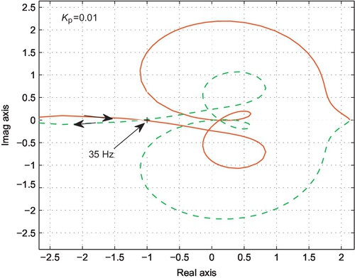
• Case 2 Kp = 0.01
The Nyquist plots are shown in Figs. 6.14 and 6.15. It is observed that when the gain is larger or equal 0.01, the Nyquist maps encircle (−1,0) clockwise, which indicates instability. The point when the curve traverses the real axis is at 35 Hz. When the gain is zero, (−1,0) is not encircled and the phase margin is 11° at 33 Hz.

Bode plots of the impedances Znet and Zsr are shown in Fig. 6.16. It is shown that a higher current controller gain increases the magnitude of Zsr and leads to a lower frequency at Znet = Zsr. The phase angle of the impedances at unit gain of Znet/Zsr are recorded in Table 6.1.

Table 6.1
Phase Angles of the Impedances and Stability Detection
| Kp = 1 | Kp = 0.1 | Kp = 0.01 | Kp = 0 | |
| Res. freq. (Hz) | 20 | 32 | 35 | 33 |
|
| − 88° | − 81.3° | − 77° | − 77° |
|
| 161° | 149° | 99.4° | 91.4° |
|
| 111° | 130° | − 178° | − 168.4° |
| Stability | N | N | Marginal | stable |

It is found that a higher gain leads to less phase margin or instability.
6.5.1.4 Validation Via Simulation
The nonlinear model presented in Chapter 5 has been built in Matlab/ Simulink. The impact of wind speed and the RSC current loop control on SSR have also been discussed. It is observed that at lower wind speed, with high compensation level, the system is subject to SSR. In this simulation study, controller interaction between the RSC’s current control and the electrical network will be verified. In [10], such phenomenon is classified as subsynchronous controller interaction (SSCI). The case study scenarios will be setup with wind speed at 9 m/s and the rotating speed at 95% of the nominal. The compensation level at 50%. The RSC control gain will be varied to show the impact of controller interaction.
• Case 2 Kp = 0.01
The system is initially operated at 25% compensation level. At t = 1 s, additional capacitors are switched in to make the compensation level reach 50%. Figures 6.17–6.19 show the dynamic responses of the system with thick lines refer to Case 1 while the thin lines refer to Case 2. The dynamic responses of the electromagnetic torque, the rotating speed of the wind turbine and the terminal voltage of the DFIG wind farm are shown Fig. 6.17. It is found that there is a resonance at about 25 Hz in the voltage magnitude and torque. For Case 1 the resonance can be damped out in the torque and the terminal voltage after 1 s. However, for case 2, the resonance cannot be damped out after 1 s.
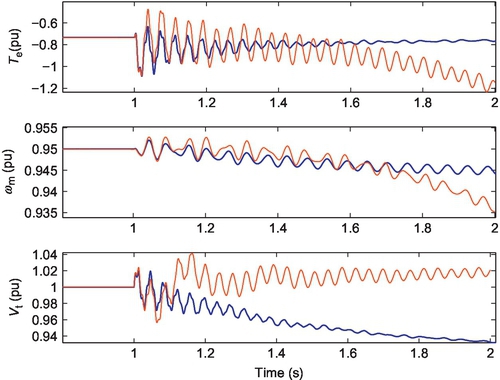

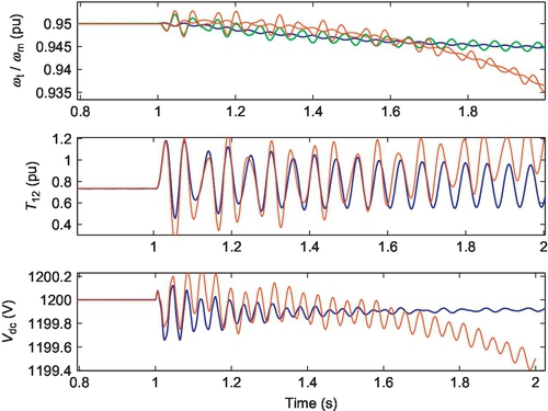
Figure 6.18 shows the dynamic responses of the DFIG wind farm output power Pe and Qe, the voltage across the capacitors Vc and the current through the line Ie. The resonance is damped out in Case 1 while persists in Case 2.
Figure 6.19 shows the dynamic responses of the rotating speeds of two masses ωt and ωm, the torque T12 between the two masses of the wind turbine and the DC-link voltage Vdc. The resonance is more obvious in Case 2. In addition, power/torque imbalance is observed that the rotating speed and the DC-link voltage keep decreasing.
According to the Nyquist/Bode analysis in Section III, the resonance is 35 Hz at 50% compensation level and 0.95 pu rotating speed. This resonance reflected in power, torque and voltage/current magnitude will have a frequency of 25 Hz. The analysis in Fig. 6.15 also shows marginal stability or instability when the gain Kp is 0.01. Simulation results demonstrate the effect of current controller gain.
6.5.2 Example 2: Impact of Unbalance Operation on SSR
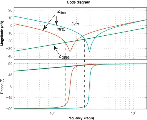
The bode plots of the negative sequence impedances are shown in Fig. 6.20. Two network impedances are presented: one is at 25% compensation level while the other is at 70% compensation level. Two DFIG impedances are presented: one is at 75% nominal speed while the other is at 95% nominal speed. From the Bode plots, the two Bode plots almost match each other. Therefore wind speed has negligible impact on the DFIG impedance. The network impedance magnitudes and the DFIG impedance magnitudes meet at 150 rad/s (24 Hz, 25% compensation level) and 250 rad/s (40 Hz, 75% compensation level). There are phase margin for Zline/ZDFIG. Hence the negative sequence impedance will not cause SSR instability.
A comparison of the positive and negative sequence impedances of the DFIG is shown in Fig. 6.21. From this figure, it is obvious that the positive sequence impedance of the DFIG could be greater than 90° at the gain cross frequencies. This indicates that it is the positive sequence impedance that could cause SSR instability.

6.5.3 Example 3: Torsional Interaction Investigation
6.5.3.1 Frequency-Domain Analysis
Bode plots of the torque/speed transfer function Gcl(s) will be plotted. The operating conditions are: wind speed 9 m/s, compensation level (25%, 50%, and 75%). Two scenarios will be examined: with positive sequence components only and with negative sequence components only. In the first case, ![]() and in the second case,
and in the second case, ![]() .
.
Figure 6.22 presents Bode plots of torque/speed relationship considering positive sequence components only. Three scenarios with different compensation levels are presented. The Bode plots indicate that the system has several oscillation modes, including a mode related to mechanical dynamics with less than 1 Hz, a mode related to the electromechanical interaction at 4-6 Hz, the subsynchronous resonance (SSR) mode (∼ 38Hz at 25%, ∼ 30Hz at 50% and ∼ 20Hz at 75%) and the supersynchronous mode. Note that the frequency of the SSR mode in torque has the complementary frequency of the SSR frequency in voltages and currents. For example, the SSR frequency of the electric system at 9 m/s at 25% compensation level is 24 Hz. The resonance frequency can be found in Figure 6.20 the phase domain impedance Bode plot. In Fig. 6.22, the SSR frequency of 9 m/s 25% case is also around 36 Hz.
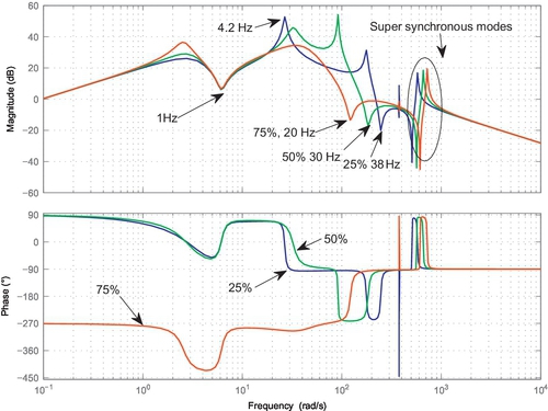
Figure 6.23 presents Bode plots of torque/speed relationship considering negative sequence components only. These Bode plots are obtained based on the linearized model where an initial negative sequence operating condition is assumed. The Bode plots in Fig. 6.22 are also shown here in dotted lines as comparison. It can be seen that magnitude wise, the negative sequence component’s effect in the range of 160 Hz is insignificant compared to the positive sequence component.

6.5.3.2 Simulation Results
In this section, time-domain simulation is carried out in Matlab/Simulink using nonlinear dq based models developed in Chapter 5. Two types of disturbances are applied to the test system where a Type-3 wind farm interconnected to a series-compensated transmission line). The parameters of the test system can be found in the Appendix of Chapter 5.
The wind speed is chosen to be 9 m/s and the system compensation level is 25%. Three cases are studied.
• In Case 1, at t = 2s, a positive sequence voltage drop (0.1 pu) is applied at the system voltage.
• In Case 2, at t = 2s, a negative sequence disturbance (0.1 pu) is applied to the system voltage.
• In Case 3, at t = 2s, a negative sequence disturbance (0.5 pu) is applied to the system voltage.
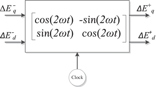
The simulation model is built in dq synchronous reference frame. In Case 1, a step response is applied at the q-axis system voltage. While in Case 2 and Case 3, a step response is applied at the q-axis of system voltage of the dq− reference frame. It is then transformed into dq+ reference frame as shown in Fig. 6.24.
The system dynamic responses will be presented. The simulation results are presented in the following figures. Figure 6.25 presents the machine rotating speed dynamic responses. It can be observed that there are SSR mode at 36 Hz and a 4.5 Hz oscillation in the balanced disturbance case. When unbalanced disturbance is applied, the 120 Hz oscillation is sustained as long as the unbalanced disturbance is presented. In addition, a 4.5 Hz oscillation is also obvious. The SSR oscillation distorts the 120 Hz oscillation as well. At 2.5 s, the distortion is no longer obvious, which indicates the die-out of the SSR mode.
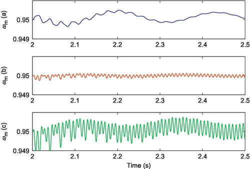
Figure 6.26 presents the torsional speed (ωt) and the intermediate torque T12 in the two-mass turbine. A much lower oscillation mode (<1 Hz) is now presented. This mode corresponds to the mechanical mode indicated in the Bode plots. The 4.5 Hz oscillation can be observed obviously. The comparison of three cases indicate that a 0.5 pu unbalanced disturbance has similar effect of 0.1 pu balanced disturbance. Regarding the effect on damping of these two modes, unbalanced or balanced disturbance does not have any noticed difference.

As a comparison, another scenario when the series compensation level is 50% is studied and the simulation results are presented in Figs. 6.27 and 6.28. Observing Case 1 in Fig. 6.27 can find that the SSR mode is now with a frequency of 27 Hz. This observation corroborates with the analysis by Bode plots in Section 6.5.3.1 (e.g. Fig. 6.22) that when series compensation level increases, the SSR mode frequency decreases in torque. Comparison of the dynamic response of T12 in Fig. 6.28 indicates that the 0.5- and 5-Hz oscillations are all presented in balanced and unbalanced cases.


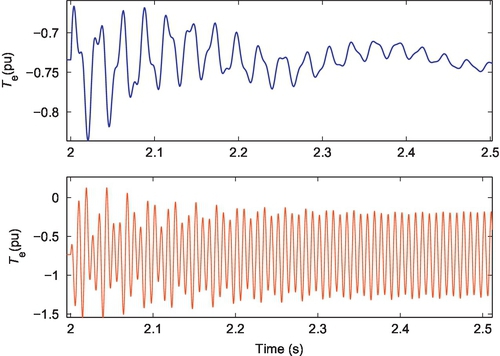
Figure 6.29 present the simulation results of electric power and electromagnetic torque. In both cases, 36 Hz SSR mode can be observed in the balanced case and unbalanced case. Though unbalanced case has sustained 120-Hz oscillation.
The above simulation results demonstrate that except an addition of 120 Hz oscillation, unbalanced disturbance does not worsen the other oscillation modes. It is also understandable that the simulation case is a small disturbance case, therefore the system characteristic will be determined by the operating point which is balanced operation.
Comparison cases also indicate that a 5 times larger unbalanced disturbance could have comparable impact as a balanced disturbance on the system if the 120 Hz oscillation is excluded.