3
Setting Up a Lumped Parameter Model
Summary
This chapter aims to offer the reader an introduction to setting up a lumped parameter model. It is often the engineer’s task to set up a model that enables the representation of a given system. An abstraction effort is therefore required, and the representation of the model to be set up will have a level of detail that depends on the type of excitation and on the intended objective. This chapter draws on an example of an electric fan power drive. It presents deduction approaches that progressively increase model complexity until achieving the intended phenomenon, as well as model reduction approaches that enable the selection of the main elements from an initially complex model.
Learning outcomes
On completing this chapter, the reader is expected to:
- – Concerning the analysis and modeling of a multi-physics system:
- - Identify the main domains (electricity, mechanics, hydraulics, heat transfer, and signal) and the system interfaces;
- - Systematically analyze (table) the various effects (transformer, storage, and dissipation) of a system;
- - Be able to evaluate the importance of an effect based on geometric criteria and on the properties of materials;
- - Set up a 0D/1D Modelica diagram of a multi-physics system;
- – Concerning the modeling approaches and the selection of adapted models:
- - Know how to adapt a model complexity level to the requirements (depending notably on the range of excited frequency);
- - Set up an increasingly complex modeling process aimed at reaching the representation of the phenomenon under study;
- - Reduce model complexity until achieving the proper model that enables phenomenon analysis or saves calculation time.
3.1. Introduction to the notion of adapted model
3.1.1. Chapter objectives and approach
This chapter aims to provide the reader with an introduction to setting up simulation models. Chapter 2 focused on the fundamental laws governing:
- – a set of components and their interaction: Kirchhoff’s laws;
- – a range of possible effects (source, dissipation, storage, and transformer effect) in various domains (electricity, hydraulics, heat transfer, or mechanics).
For the examples that have already been studied, the elementary effects and the values of the corresponding parameters were known. Here, the aim is to determine the elementary effects to be considered for the representation of the phenomenon to be studied. As will be seen, the model to be set up depends, in particular, not only on the system’s topology but also on the type of excitations it will undergo and on the objective of the study.
The approach taken here to set up an adapted model can be described as follows:
- – Analyze the topology or the geometry of the system to be modeled to identify the possible effects to be considered. These effects must be known and a choice must be made among them prior to simulation.
- – Make sure that the model built has the proper precision level to represent the phenomenon under study. An incremental modeling approach based on the most elementary effects may ensure the proper modeling level.
- – Reduce model complexity level by ignoring negligible effects. If the initial model is relatively complex, its simplification may speed up the simulation process, for example, in case of real-time simulation. Furthermore, model simplification may contribute to a better understanding of the phenomena to be studied, for example, in the design phase.
3.1.2. Problem under study
In order to illustrate these various concepts, a guideline example will be used throughout this chapter: the starting of a high-power electric fan. This type of electric fan is present in some cooling towers of electric power plants (Figure 3.1). The coolant is the endpoint of the cooling circuit in which heated water is cooled by an ascending flow of cool air. These induced flow cooling towers [HAM 18] tend to replace the classical atmospheric cooling towers of power plants, on the grounds of visual impact and control flexibility.

Figure 3.1. Cooling towers of electric power plants
As shown in Figure 3.2, the electric fan located at the top of the tower includes an induction motor, a driveshaft, a reducer, and the fan blades. The motor is directly connected to the network through power contactors and protection elements. It has no variable speed drive and, therefore, runs in steady state at a fixed speed, except when starting. As the remainder of this chapter highlights, a poor model choice may lead to undersizing during the selection of components and explain, for example, the possible short service life of the reducers employed in such applications.
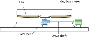
Figure 3.2. Motor-fan group
3.1.3. Importance of the type of excitation
Simulation models can be more or less precise, depending on the type of excitation:
- – For relatively slowly varying phenomena, the system can be assumed to operate in steady state or in quasi-static state. Quantities resulting from derivatives with respect to time are in this case negligible and state variables can be considered constant. Models can be reduced to source, transformer, and dissipative effects. Mathematical processing involves only algebraic equations that can be implemented in many computation environments;
- – When mission profiles vary more rapidly, consideration of certain dynamic effects may be required, such as rotor inertia generating additional forces in relation to its acceleration. If only one type of energy storage is involved, responses exhibit no resonance phenomena;
- – If very rapid transient variations are manifest, resonance modes can be excited and significant oscillations can be added to the variables. These resonance modes are due to the interaction of several types of energy storage elements.
The electrical example in Figure 3.3 illustrates the possibility to use more or less detailed representations depending on the frequency and type of excitation. Here the objective is to simulate the current absorbed by the load depending on the applied voltage. It is worth noting that for low- or high-frequency voltages, the diagram can be simplified while the absorbed current is accurately represented. The response of the simplified diagrams is always compared in the graphics (Figure 3.3.d and f, superposed red and blue curves) with that of the complete diagram.
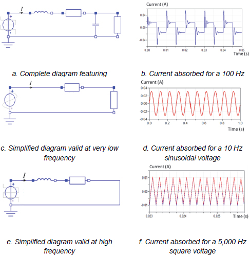
Figure 3.3. Current in an electric circuit for various waveforms and frequencies
3.2. Identifying the main effects
3.2.1. Systematic setup of domains and effects
As a first step in the modeling process, a table may be used in the systematic search for effects to consider in the overall representation of the system. Table 3.1, represented below, has three columns: the first one for components or subsets to be represented, the second one indicating the domain (mechanics/electricity/…) to which these components belong, and the last one to indicate the source/transformer, storage or dissipative effects that may be identified. The choice of the latter effects requires analytical skills that the reader may acquire by solving the small exercises suggested at the end of the chapter.
Table 3.1. Systematic analysis of effects
| Main and parasitic effects | ||||
| System component or subset | Domain | Source or transformer | Energy storage | Dissipation |
| Electric network | Electricity | Voltage source | ||
| Electric motor | Electricity and mechanics (rotation) | Electromechanical transformer | Winding inductance Rotor inertia |
Winding resistance Bearing friction |
| Driveshaft | Mechanics (rotation) | Inertia, shaft stiffness | Internal damping | |
| Reducer | Mechanics (rotation) | Reduction ratio | Pinion inertia, tooth stiffness | Reducer efficiency |
| Fan | Mechanics (rotation) | Source of aerodynamic forces (function of rotational speed) | Blades inertia | |
3.2.2. From geometry to network
As noted earlier, the simplest model often includes only the device transformer and dissipative effects. The latter may have nonlinearities that are beyond the scope of this chapter. Chapter 6 will show how the nonlinearities of certain transformer effects in mechanics (nonlinear kinematics) or in electrical engineering (electromagnet) can be modeled. A more detailed model should integrate energy storage elements. The analysis of the geometric and material configuration of the device may help in finding the dominant effects. A mechanical system such as the electrical fan requires the identification of the main inertias and elasticities of the device.
In the rotational domain, under the action of a torque, inertia limits acceleration and elasticity causes angular deformation. It is therefore important to identify the elements with significant inertia and those with low stiffness. Unlike the software tools for distributed parameter modeling, which rely, for example, on finite elements, and make it possible to directly represent a geometry close to reality, lumped parameter modeling requires additional abstraction. For a shaft composed of cylinder elements, inertia and stiffness can be approximated by the following formulae:
- – Inertia of a cylinder of mass M and radius r:
- – Torsional stiffness of a tube of length L, outer and inner diameters dext and dint, and shear modulus G:
[3.2]

Hence, a driveshaft with a small diameter and a significant length has low inertia and low stiffness; therefore, only stiffness is retained for its modeling. The motor rotor with the most significant diameter will be represented by inertia.
Figure 3.4 shows a simplified 3D geometric representation of the fan/rotor/driveshaft set and its equivalent in 0D/1D modeling. This lumped parameter representation assumes that reducer inertia and elasticity are negligible (particularly with respect to motor inertia and driveshaft elasticity).

Figure 3.4. From the geometric model to the lumped parameter model
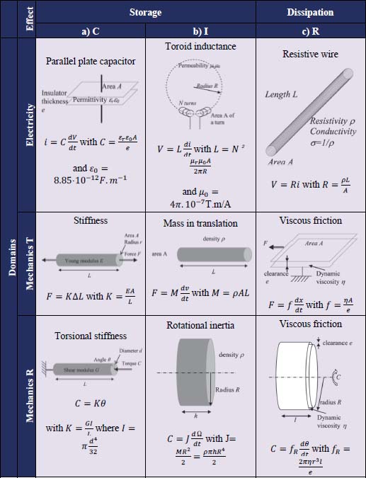
Table 3.2 presents a summary over various domains of the expressions of parameters associated with elementary geometries. The reader can use it to refine the analytical skills required to recognize these effects.
Table 3.2. Analytical expressions of the parameters for elementary geometries

3.3. Modeling approaches and selection of adapted models
As described in the Introduction, these effects will be added in ascending order of complexity. The objective is to determine the mechanical actions through the shaft upon the start to validate the choice of components, particularly that of the reducer. The aim is to determine the model that meets the basic requirements for understanding the dominant interactions.
3.3.1. Incremental modeling by increasing complexity
The deductive approach progressively refines the model until reaching the appropriate level: the components are first represented by their ideal operational behavior, and imperfections are added to represent the phenomena with increasingly small time constants. For the case study considered here, the objective is to represent the torques through the reducer to explain the particularly small service lifetimes observed in practice. Figure 3.5 presents these increasingly complex modeling levels:
- a) The first quasi-static modeling level represents only the characteristics of motor torque/speed and of the load, as well as the reducer with its transformation ratio and its efficiency. This model can only represent the steady state torque and speed after the start.
- b) The second level represents the inertia of the motor and the blades and facilitates the representation of the acceleration and of the maximal torque of the asynchronous motor during the starting phase.
- c) The third level takes into account the driveshaft elasticity, which may enable the visualization of the oscillations of inertias.
- d) The last level takes into account the electrical stator and rotor time constants.

Figure 3.5. Various modeling levels for the motor fan
Figure 3.6 shows the simulation results for the torque and the speed on the high-speed axis of the reducer for a), b), and c) modeling levels in Figure 3.5. It can be noted that the results in steady state at constant speed are similar for all modeling levels. Nevertheless, during the start, the maximal torque depends significantly on the chosen model. Considering inertias facilitates the representation of a starting torque surge due to the torque–speed characteristic of the induction motor. The model that takes into account the driveshaft stiffness generates an even stronger transient torque. It, therefore, seems that the representation of the mechanical resonance mode is essential. This mode is excited by the sudden rise in motor torque upon direct connection to the electrical network, as well as by the negative damping characteristic of the first part of the torque/speed curve of the induction motor. Chapter 5 provides the mathematical tools for analyzing these phenomena. The last level d) in Figure 3.5 (not represented here) provides no additional information for this maximal torque. The model that is just sufficient here is, therefore, c) level in Figure 3.5.

Figure 3.6. Simulations of various modeling levels (high-speed axis of the reducer)
3.3.2. Model reduction by activity index analysis
The previous section has highlighted torques oscillating with high amplitudes during the start. They require very strong oversizing of the reducer with respect to the torque to be provided in the steady state. Even the use of a 4 or 5 safety factor cannot avoid rapid deterioration of the reducer if the designer uses only model a) in Figure 3.5 to select this component. These usage constraints can be limited if resonance mode excitation is avoided. This requires the use of a starting torque that has no sudden discontinuity. This progressive starting can be obtained by driving the induction motor at variable speed by means of a static converter. This costly electronics device offers the additional function of a speed that can be controlled in the steady state for accurate control of the electric power plant operation.
The high starting torque of an induction motor can be reduced if a sloped speed profile with no discontinuity is applied by a speed control unit. Figure 3.7 shows the corresponding model in which a speed control unit can be represented by a Proportional Integral (PI) controller or by inverse simulation. Figure 3.8 shows the simulation results for these models.
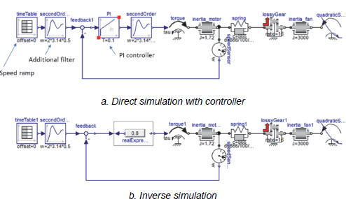
Figure 3.7. Mechanical modeling of a variable speed motor fan

Figure 3.8. Speed and torque evolution for a progressive rise in speed within 10 s
Inverse simulation avoids the need to design the controller with the expected performance by imposing a zero error directly between the set-point and the actual speed. The two models produce the same results. Figure 3.8 shows that the maximal torque applied to the reducer has a much lower value in this case compared to the previous architecture. Torque oscillations are also significantly reduced.
The next question to be addressed is whether it is possible to reduce model complexity while preserving an acceptable prediction in view of the reducer choice. Generally speaking, the model reduction approach starts with a very detailed model and preserves only the elements with the strongest influence on the response of the model. Literature [ERS 08] classifies the reduction techniques into approaches based on the frequency behavior and analyses based on energy. Only energy-based methods are studied here, as they can be directly applied to the lumped parameter without needing to determine the frequency representation (transfer function) or the state space (matrix) of the models. Chapter 5 illustrates the use of these latter representations. Energy-based techniques assume that the components that weigh the most in the precise modeling of a system are characterized by the largest amplitudes of energy flow. This amplitude, which is also known as the activity of an element or component, results from the integration of the absolute value of the power flowing through it over a specific time window and for a specific input. Therefore, the activity of an element Ai is defined as follows:
where e and f are power variables (effort and flow) and characteristics of the element such as force/speed in mechanics and voltage/current in electricity.
This measure, proposed by L. S. Louca [LOU 98], is directly involved in certain environments such as AMESim. In Modelica environments, it can be implemented in the form of sensors as shown in Figure 3.9. These sensors have been used for measuring the activities of inertia and stiffness in Figures 3.5.c and 3.6. The various activities (all positive) are then compared in percentage with their total sum in Table 3.3. It is worth noting that the activity of the driveshaft stiffness decreases particularly starting with an electronic speed controller. It, therefore, seems possible to eliminate the stiffness element from the diagram. Figure 3.10 compares the simulations of torque and speed on the high-speed driveshaft by considering or neglecting this stiffness. Speed profiles are superimposed. In the absence of the shaft stiffness, the low-amplitude oscillations disappeared from the response of the direct starting. Since the model involves only inertias, it could be sufficient for the selection of the reducer or for making an HIL simulator of the physical system.
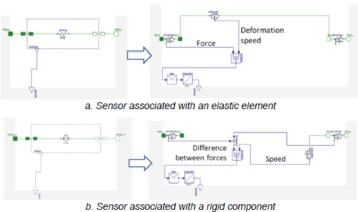
Figure 3.9. Sensors of the activity index
Table 3.3. Activity index of the models with and without a controller
| Direct starting on the network by contactors | Controller-based starting (10 s of speed rise) | |
| Fan inertia | 46.7% | 87.7% |
| Driveshaft stiffness | 9% | 0.3% |
| Motor inertia | 44.3% | 12% |

Figure 3.10. Torque/speed for various model levels (with and without driveshaft stiffness)
3.3.3. Model reduction by design of the experiment or by comparison of effects
Although interesting, the activity index approach is not always implemented in a standard manner in multi-physics modeling software. Therefore, it may be quite difficult to implement, requiring specific additional sensors. Other analysis techniques are nevertheless available.
The first relies on Design of Experiments (DoE) [MON 17] and on the sensitivity analysis of simulation models. Many platforms propose parameter variation tools that can be used to estimate the effect of one or several parameters. The simple approach used here involves a disturbance applied according to a method referred to as One at a Time [ELM 05]. The model in Figure 3.7 is simulated for rated values of the motor inertia parameters, fan inertia, and driveshaft stiffness and their 10% variation. The torque on the high-speed axis of the reducer is then displayed, as shown in Figure 3.11, for various experiments. For this problem, the most influential parameter is fan inertia. It can also be noted that motor inertia has a small influence on the reducer torque. In fact, control imposes motor speed, and torque transients are functions only of the driveshaft stiffness and of the blade inertia. It can also be noted that stiffness variation has a very small effect on maximal torque.
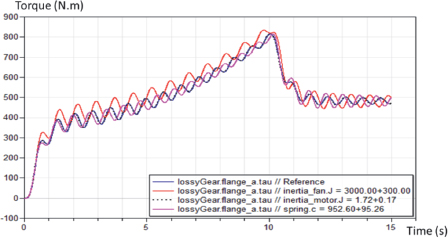
Figure 3.11. Simplification of the model by design of experiments
The last approach presented here does not require any tool or simulation. It involves a direct comparison of the values of parameters to evaluate their importance in the problem at hand. This may require the determination of the equivalent parameters, as illustrated in Figure 3.12 for fan inertia. An equivalent parameter can be determined around a power transformer component as follows:
- – By direct processing of the characteristic equations: for inertia on the low-speed axis (index LS) of a reducer, with reducing ratio N, the torque/acceleration expression is:
The introduction of speed and torque on the high-speed axis (index HS) gives:
which highlights the equivalent inertia on the high-speed axis:
- – By equality of stored energy or of dissipated power by the equivalent component: the stored kinetic energy must be identical in the two configurations shown in Figure 3.12, which gives:
Generally speaking, the equivalent parameter reveals the squared transformation ratio of the transformer. The transformer can connect different domains, as an electric motor connects electrical and mechanical domains, and reveals parameters of various natures, such as inductance or capacitance.
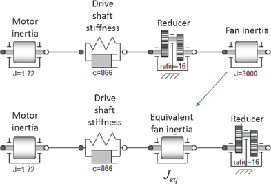
Figure 3.12. Setting up an equivalent component
The equivalent fan inertia calculated here on the high-speed axis of the reducer is 11.72 kg.m2, which is more than that of the motor, 1.72 kg.m2. But model simplification requires, first of all, the evaluation of the importance of the presence of stiffness K of the driveshaft and particularly its possible interaction before the equivalent inertia. It can be quantified by the resonance frequency calculated here assuming that the potential effect of motor inertia is neutralized by speed control:
which here is 1.4 Hz. Depending on the spectral diversity of the speed profile, which can be controlled by the second-order filter located upstream of the speed set point, this resonance mode can be excited. Figure 3.13 illustrates two different cases, below and above 1.4 Hz, and shows the advantage of using a filtered speed set point to avoid resonance mode excitation. In this latter case, the effect of the driveshaft elasticity can be neglected when sizing the reducer.
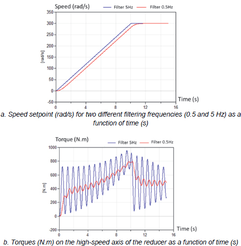
Figure 3.13. Influence of the spectral content of the speed set point
3.4. Introductory exercises related to setting up models with lumped parameters
The exercises in this section are designed as an introduction to setting up models with lumped parameters. Multi-physics modeling requires the formulation of modeling hypotheses that may sometimes be quite strong, but enable capturing the main effects to be represented. In contrast to the previous chapter, the effects and parameters are not given: they must be determined based on the textual or geometric description of the devices.
3.4.1. Building up analytical skills
3.4.1.1. Storage and dissipative effects
Lumped parameter modeling involves abstraction and choice of the main effects to be represented. Therefore, it requires knowledge of the considered domains. Table 3.2 summarizes, for elementary geometries, the storage and dissipative effects and the expressions of the associated parameters.
Table 3.4. Multiple-choice table corresponding to question 1
| Domain | Effect | |||||||
| Electricity | Mechanics T | Mechanics R | Hydraulics | Heat transfer | C a) | I b) | R c) | |
| a | b | c | d | e | f | g | h | |
| 1. Conductive elements separated by a dielectric. | ||||||||
| 2. Surfaces in contact and in relative motion. | ||||||||
| 3. Massive rigid body. | ||||||||
| 4. Long wire of small cross-sectional area. | ||||||||
| 5. Poor heat conductor volume of low density. | ||||||||
| 6. Set of many conductive turns in a small volume. | ||||||||
| 7. Pipe blocked at one end and subjected to increasing pressure at the other end. | ||||||||
| 8. Heavy mass of uniform temperature. | ||||||||
| 9. Light body with a temperature gradient. | ||||||||
| 10. Large diameter rotating part. | ||||||||
| 11. Deformable blade. | ||||||||
| 12. Long pipe of small cross-sectional area. | ||||||||
| 13. Large volume of compressible fluid. |
The objective is to help the reader develop his or her analytical skills required to identify these effects.
- 1. Depending on the phenomenon to be modeled, check in the following table the physical domain and the type of effect to consider.
NOTE.– C, I, or R are notations used for the elementary effects, as employed in the bond-graph approach that will be presented in Chapter 4. C and I effects or elements store the energy. With the exception of heat transfer, the R element dissipates energy in the form of heat. An I element stores energy in a state variable representing motion or speed (mechanical speed, electric current, hydraulic flow rate, etc.) while a C element stores energy in a static state variable (force, voltage, pressure, etc.).
- 2. For the technical devices represented in the following, indicate the dominant effect for each part from a) to e):
- – Accelerometer: Figure 3.14 represents a MEMS accelerometer (Micro Electro Mechanical System). This microscopic device is made from silicon by etching a superficial layer through a chemical process to obtain a moving part.
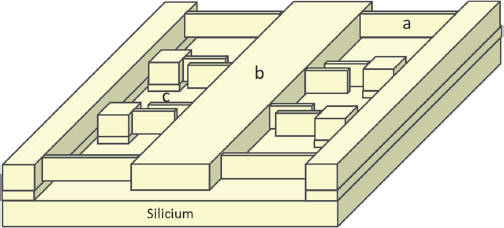
Figure 3.14. MEMS accelerometer
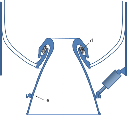
- – Launcher booster nozzle: this nozzle has two rotational degrees of freedom for the control of thrust direction of propellant gases.
3.4.1.2. Transformer effects
The ideal behavior of many power transmission components is assimilated to a transformer effect that does not store nor degrade the transferred energy. They are characterized by a set of two equations connecting the power variables.
An ideal direct current motor is modeled by a set of equations:
with:
- – Torque C and speed ?, power variables on the mechanical port;
- – Voltage E and current I, power variables on the electrical port.
- 3. Prove that transformation ratios kc and kE are identical.
- 4. Fill in Table 3.5 by indicating the components and the equations corresponding to the following devices (Figure 3.16.a and b). Focus on the underlined components and on their modeling in the form of ideal transformers without losses and without energy storage (two equations per component).
Table 3.5. Table to be filled corresponding to question 4
| DC Elec | |||||
| AC Elec | |||||
| Mecha T | |||||
| Mecha R | |||||
| Hydro | |||||
| DC Elec | AC Elec | Mecha T | Mecha R | Hydro |
- – EHA (Electro-Hydrostatic Actuator) flight controls;

Figure 3.16.a. EHA flight controls
- – Electric elevator power drive of direct current motor/chopper type;

Figure 3.16.b. Electric elevator power drive
3.4.2. Geometry/network link: power steering analysis
Figure 3.17 describes the implementation and the general and detailed architecture of a Renault Twingo electric power steering.

Figure 3.17. Renault Twingo electric power steering
Figure 3.18 shows the Modelica diagram modeling this power steering.
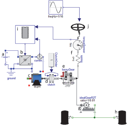
Figure 3.18. Modelica diagram of Twingo electric power steering
- 1. In Table 3.6, circle the Modelica component (a, b, c, d, e, f, g, h, i, or j) corresponding to the physical component. Name each component.
- 2. Suggest a Modelica diagram that models the direct current motor (component c of the global Modelica diagram) and takes into account the energy transformer, dissipative and storage effect both at mechanical and electrical levels.

Table 3.6. Multiple-choice table corresponding to question 1
- 3. Here is a modeling proposition for the tie rod–wheel pivot–tire set (component h on the global Modelica diagram). Identify in the diagram the effects represented by each Modelica component.

3.4.3. Systematic analysis of effects: analysis of a direct injection system by common rail
Direct injection systems by common rail use piezoelectric or electromagnetic injectors to enable the very precise control of the quantity and chronology of fuel injection in each cylinder of an internal combustion engine. This type of injector is electrically controlled, therefore software can be embedded in this technology. A direct injection system with common rail, represented in Figure 3.20, is composed of a low-pressure fuel boosting pump followed by a high-pressure pump, driven by the motor, which fuels the common rail; a pressure relief valve, which controls the common rail pressure; a hydraulic accumulator, known as common rail, which constitutes a high-pressure fuel reserve for the injectors; and an injector per cylinder, playing the role of electro-hydraulically controlled valves.
- 1. A global model of the system can be used, for example, for pressure stability evaluation. Fill in the following analysis table describing the main domains and effects enabling the modeling of each component of the system:
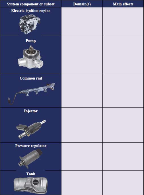

Figure 3.20. General diagram of a direct injection system by common rail
3.5. Problems related to the choice of modeling level
3.5.1. Thermal response of a TGV motor – deductive approach
V150, a special TGV high-speed train, has set a speed record of 574.8 km/h on the railway on April 3, 2007, on East Paris–Strasbourg line. The previous record of 513.3 km/h had been achieved in 1990. The test train, schematically shown in Figure 3.21, included on that occasion TGV POS power cars (TGV Est lines, POS for Paris – Ostfrankreich – Süddeutschland), AGV (from the French Automotrice à Grande Vitesse, self-propelled carriages), and high-speed rail motor cars, and was expected to exceed 150 m/s (or 540 km/h).
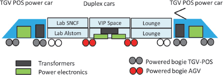
Figure 3.21. V150 test train set [ALS 08]. For a color version of the figure, see www.iste.co.uk/budinger/multiphysics.zip
AGV rail motor cars have bogies (Figure 3.22) powered by permanent magnet synchronous motors. Each motor has a nominal power of 700 kW and has been used during a short-term overload at 1 MW to break the speed record. An electric motor can significantly degrade if heat due to Joule losses induces very high temperatures in the winding insulation. A thermal model will be built to estimate the maximum overload time of these motors.
Nominal motor characteristics at 700 kW are as follows:
- – Nominal torque Cnom= 1400 N.m for a nominal speed ?nom = 4,800 rev/min;
- – Joule losses corresponding to this operating point PJ, = 5 kW;
- – 140°C increase in winding temperature above an ambient temperature of 40°C.
- 1. Motor overuse is manifest at the torque level preserving a maximal speed of 4,800 rev/min (by reducer adaptation). Calculate the motor torque during the speed record.
- 2. Calculate the corresponding Joule losses. It is worth recalling that torque is proportional to current.

Figure 3.22. Powered bogies of AGV rail motor cars
- 3. Suggest two modeling levels and draw the corresponding thermal nodal diagrams. The first level assumes that the motor is equivalent to a single body of uniform temperature, while the second level differentiates between winding temperature and iron core temperature.
- 4. Based on the information provided in the text or in Figure 3.23, suggest values for the parameters in these diagrams.
- 5. Implement these models under Modelica, and simulate rated operation and worldwide record operation. Joule losses take the temporal form of a step.
- 6. Deduce from the simulations at each level of the model the time available to break the worldwide record. What is the least conservative model to be used for this time estimation?

Figure 3.23. Simplified cross-sectional view of a synchronous motor stator
3.5.2. Modeling of a power steering torque sensor – geometry analysis
An electric power steering has a torque sensor located on the steering shaft between the steering wheel and the electric assistance motor drive. The electric motor torque is controlled depending on the torque provided by the driver and measured by this sensor. The objective of this problem is to analyze a sensor employing magnetic technology, which enables torque measurement without contacting a rotating shaft.
Figure 3.24 shows a cross-sectional view of the torque sensor of Twingo electric power steering. This sensor has three parts:
- – The mechanical part (Figure 3.24.a in green) includes a torsion bar, which can be modeled by a specific value of torsion stiffness and induces an angular displacement between the input shaft and the output shaft that is proportional to the torque applied by the driver;
- – The electromagnetic part (Figure 3.24.a, in yellow with A and B marks, and schematically represented in Figure 3.24.b) of the sensor provides information on the angular position error of the detection rings (A and B) and consequently of the input shaft (steering wheel side) with respect to the output shaft (steering side);
- – The electronic part of the sensor transforms the information referring to the modification of angular error measured by A and B windings into torque information represented by a voltage.

Figure 3.24. Cross-sectional view of the power steering torque sensor and principle of the magnetic part
The electromagnetic part has two windings (A and B), each inducing a magnetic field in a magnetic circuit partially made of rings A and B connected to the steering shaft. Figure 3.25 shows an axisymmetric 2D finite element magnetic simulation of the winding/ring set A. The magnetic field lines represent the direction of the magnetic field ![]() . Their density expresses field intensity. In what follows, our modeling will ignore the magnetic field lines in the form of a quarter of a circle constituting the leakage flux of the magnetic circuit. The magnetic flux ? can be calculated by integration of the magnetic field over a surface:
. Their density expresses field intensity. In what follows, our modeling will ignore the magnetic field lines in the form of a quarter of a circle constituting the leakage flux of the magnetic circuit. The magnetic flux ? can be calculated by integration of the magnetic field over a surface:
Several laws can be used for magnetic circuit modeling:
- – Magnetic flux conservation expressed by
 over a closed curve;
 - – Ampère’s circuital law
 connecting the intensity of the magnetic field on a loop and the intensity of the current I enclosed by this loop. The winding of N turns increases induction;
 - – Lenz’s law
 expressing the voltage induced in a winding of N turns by the variation of flux across it.
It is possible to represent the behavior of a magnetic circuit using laws similar to Kirchhoff’s laws. The equivalent of the electric current is magnetic flux.
- 1. What physical law here expresses Kirchhoff’s voltage law? Answer the same question for Kirchhoff’s current law. What physical quantity is equivalent to voltage?
- 2. Find the expression of equivalent resistance (called reluctance).
- 3. Figure 3.26 shows the lumped parameter representation of part A of the sensor. Explain what components a, b, c, d, and T in Figure 3.26 represent in Figure 3.25.
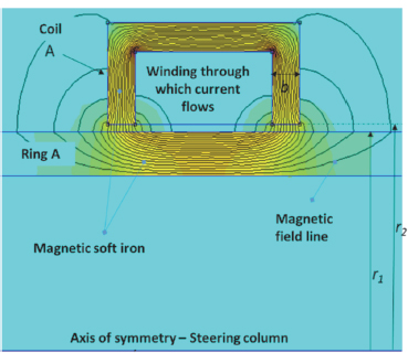
Figure 3.25. 2D finite element simulation of the magnetic field of part A of the sensor
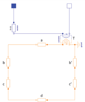
Figure 3.26. Lumped parameter modeling of part A of the sensor
- 4. Assuming that permeability ? of soft iron parts is infinite, find the expression of inductance L of the sensor as a function of air permeability µ0, number N of winding turns, radii r1 and r2, and width b. Find the numerical expression of L for r1= 15 mm, r2 = 16.5 mm, b = 2 mm, N = 1,000, and µ0 = 4 ?. 10–7 SI.
- 5. Use simulations to compare the behavior of the winding model in Figure 3.26 to an impedance RL using the inductance L calculated earlier. For the two models, the winding resistance is assumed to be equal to 30 Ω.
Figure 3.27 describes the global model of the torque sensor. It includes three domains: mechanical on the left part, magnetic for components A and B, and electronic/signal for the rest. Component A corresponds to Figure 3.26.
- 6. What does the rotational stiffness correspond to in the diagram in Figure 3.27?
- 7. How should the diagram in Figure 3.26 be modified to obtain component B? A new magnetic component might be needed.
- 8. This sensor electronic conditioning is similar to that of a Wheatstone bridge. This bridge is supplied by a sinusoidal voltage source of 5 kHz. Explain the role of the multiplier and of the low-pass filter.
- 9. Use simulation to test the operating principle of this sensor (be sure to precisely define the simulation duration and the number of measurement intervals). What conditioning function should be added to have a functional torque sensor?
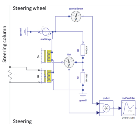
Figure 3.27. Torque sensor modeling
3.5.3. Calculation of the short-circuit torque of a submarine propulsion motor – model reduction
Diesel (non-nuclear) attack submarines often have a diesel-electric propelling system with generators driven by diesel motors and an electric motor that directly drives only one propeller. Battery recharge by diesel engines must be done just below the surface (periscope). Figure 3.28 shows some of these components such as alternators or the propulsion motor on the synthetic diagram in Figure 3.29.
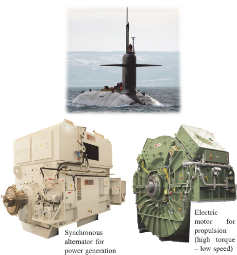
Figure 3.28. Alternator and electric motor for the navy (courtesy of Jeumont Electric [JEU 18])
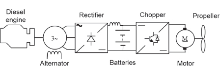
Figure 3.29. Technological diagram of the propelling set
The objective in the following is to implement the transient simulation enabling the calculation of the short-circuit torque of the electric motor. This situation is a sizing scenario for the driveshaft and makes it possible to verify that its integrity is preserved during an attack that may cause an electric failure.
The shaft line presented in Figure 3.30 transfers mechanical power from the electric motor to the propeller. Its main components are an electric motor, a hollow shaft, a seal, bearings, and end-stops enabling thrust transfer from the propeller to the submarine structure.

Figure 3.30. Shaft line between electric motor and propeller
In what follows, the hypotheses used are:
- – The coupling between the submarine forward movement and the propeller torque is ignored. The torque/speed characteristic of the propeller is approximated using a quadratic law such as T = αΩ2;
- – The diesel generator sets are not modeled. The electric motor is assumed to be supplied by a bus whose voltage ranges between 0 and Umax depending on the forward speed;
- – The temporal profile of the motor voltage supply is the following: ramp from 0 V to Umax for 200 s, plateau at Umax for 200 s, sudden shift (short-circuit) from this voltage to 0 V at the instant t = 400 s, and plateau at 0 V for 200 s.
- 1. Suggest and implement a model having the set of characteristics useful for modeling the shaft line. Some parameters that have not been directly provided can be approximated by simple reasoning.
- 2. Simulate a short-circuit using the previously given supply profile. Find the value of the maximal transient torque. Compare this short-circuit torque to the motor rated torque.
| Electric motor | |
| Rated torque | 1.75.105 N.m |
| Rated speed | 120 rpm |
| Rated voltage | 700 V |
| Resistance | 8 mΩ |
| Inductance | 20 mH |
| Rotor inertia | 3.103 kg.m2 |
| Viscous friction | 10 N.m/(rad.s−1) |
| Mass | 45 tonnes |
| Propeller | |
| Diameter | 6 m |
| Mass | 41 tons |
| Inertia | 150.103 kg.m2 |
| Shaft | |
| Diameter | 25 cm |
| Length | 4.5 m |
| Stiffness | 6.5.106 N.m/rad |
| Inertia | 20 kg.m2 |
| Viscous friction equivalent to internal damping | 25,000 N.m/(rad.s−1) |
| Seal | |
| Dry friction torque | 9000 N.m |
3. For a better understanding of the origin of this transient, the most important components to be preserved must be identified without significantly altering the simulation results. Suggest a model analysis and simplification approach for this purpose. After implementation, identify the nature of the components generating this transient torque.