Recipe 1. One-hot encoding
Recipe 2. Count vectorizer
Recipe 3. n-grams
Recipe 4. Co-occurrence matrix
Recipe 5. Hash vectorizing
Recipe 6. Term frequency-inverse document frequency (TF-IDF)
Recipe 7. Word embedding
Recipe 8. Implementing fastText
Recipe 9. Converting text to features using state-of-the-art embeddings
Now that all the text preprocessing steps have been discussed, let’s explore feature engineering, the foundation for natural language processing. As you know, machines or algorithms cannot understand characters, words, or sentences. They can only take numbers as input, which includes binaries. But the inherent nature of textual data is unstructured and noisy, which makes it impossible to interact with machines.
The procedure of converting raw text into a machine-understandable format (numbers) is called feature engineering. The performance and accuracy of machine learning and deep learning algorithms are fundamentally dependent on the feature engineering technique.
This chapter discusses different feature engineering methods and techniques; their functionalities, advantages, and disadvantages; and examples to help you realize the importance of feature engineering.
Recipe 3-1. Converting Text to Features Using One-Hot Encoding
One-hot encoding is the traditional method used in feature engineering. Anyone who knows the basics of machine learning has come across one-hot encoding. It is the process of converting categorical variables into features or columns and coding one or zero for that particular category. The same logic is used here, and the number of features is the number of total tokens present in the corpus.
Problem
You want to convert text to a feature using one-hot encoding.
Solution
I | love | NLP | is | Future | |
|---|---|---|---|---|---|
I love NLP | 1 | 1 | 1 | 0 | 0 |
NLP is future | 0 | 0 | 1 | 1 | 1 |
How It Works
There are many functions to generate one-hot encoding features. Let’s take one function and discuss it in depth.
Step 1-1. Store the text in a variable
Step 1-2. Execute a function on the text data
The output has four features since the number of distinct words present in the input was 4.
Recipe 3-2. Converting Text to Features Using a Count Vectorizer
The approach used in Recipe 3-1 has a disadvantage . It does not consider the frequency of a word. If a particular word appears multiple times, there is a chance of missing information if it is not included in the analysis. A count vectorizer solves that problem. This recipe covers another method for converting text to a feature: the count vectorizer.
Problem
How do you convert text to a feature using a count vectorizer?
Solution
A count vectorizer is similar to one-hot encoding, but instead of checking whether a particular word is present or not, it counts the words that are present in the document.
I | love | NLP | is | future | will | learn | In | 2month | |
|---|---|---|---|---|---|---|---|---|---|
I love NLP and I will learn NLP in 2 months | 2 | 1 | 2 | 0 | 0 | 1 | 1 | 1 | 1 |
NLP is future | 0 | 0 | 1 | 1 | 1 | 0 | 0 | 0 | 0 |
How It Works
The fifth token, nlp, appears twice in the document.
Recipe 3-3. Generating n-grams
In the preceding methods, each word was considered a feature. There is a drawback to this method. It does not consider the previous words and the next words to see if it would give a proper and complete meaning. For example, consider the phrase not bad. If it is split into individual words, it loses out on conveying good, which is what this phrase means.
As you saw, you could lose potential information or insights because many words make sense once they are put together. n-grams can solve this problem.
Unigrams are the unique words present in a sentence.
A bigram is the combination of two words.
A trigram is the combination of three words. And so on.
Unigrams: “I”, “am”, “learning”, “NLP”
Bigrams: “I am”, “am learning”, “learning NLP”
Trigrams: “I am learning”, “am learning NLP”
Problem
Generate the n-grams for a given sentence.
Solution
There are a lot of packages that generate n-grams. TextBlob is the most commonly used.
How It Works
Follow the steps in this section.
Step 3-1. Generate n-grams using TextBlob
There are three lists with two words in an instance.
Step 3-2. Generate bigram-based features for a document
The output has features with bigrams; in the example, the count is 1 for all tokens. You can similarly use trigrams.
Recipe 3-4. Generating a Co-occurrence Matrix
Let’s discuss a feature engineering method called a co-occurrence matrix.
Problem
You want to understand and generate a co-occurrence matrix.
Solution
A co-occurrence matrix is like a count vectorizer; it counts the occurrence of a group of words rather than individual words.
How It Works
Let’s look at generating this kind of matrix using NLTK, bigrams, and some basic Python coding skills.
Step 4-1. Import the necessary libraries
Step 4-2. Create function for a co-occurrence matrix
Step 4-3. Generate a co-occurrence matrix
I, love, and is, nlp appeared together twice, and a few other words appeared only once.
Recipe 3-5. Hash Vectorizing
A count vectorizer and a co-occurrence matrix both have one limitation: the vocabulary can become very large and cause memory/computation issues.
A hash vectorizer is one way to solve this problem.
Problem
You want to understand and generate a hash vectorizer.
Solution
A hash vectorizer is memory efficient , and instead of storing tokens as strings, the vectorizer applies the hashing trick to encode them as numerical indexes. The downside is that it’s one way, and once vectorized, the features cannot be retrieved.
How It Works
Let’s look at an example using sklearn.
Step 5-1. Import the necessary libraries and create a document
Step 5-2. Generate a hash vectorizer matrix
It created a vector of size 10, and now it can be used for any supervised/unsupervised tasks.
Recipe 3-6. Converting Text to Features Using TF-IDF
Let’s say a particular word appears in all the corpus documents. It achieves higher importance in our previous methods, but that may not be relevant to your case.
TF-IDF reflects on how important a word is to a document in a collection and hence normalizes words that frequently appear in all the documents.
Problem
You want to convert text to features using TF-IDF.
Solution
Term frequency (TF) is the ratio of the count of a particular word present in a sentence to the total count of words in the same sentence. TF captures the importance of the word irrespective of the length of the document. For example, a word with a frequency of 3 in a sentence with 10 words is different from when the word length of the sentence is 100 words. It should have more importance in the first scenario, which is what TF does. TF(t) = (Number of times term t appears in a document) / (Total number of terms in the document).
Inverse document frequency (IDF) is a log of the ratio of the total number of rows to the number of rows in a particular document in which a word is present. IDF = log(N/n), where N is the total number of rows, and n is the number of rows in which the word was present.
IDF measures the rareness of a term. Words like a and the show up in all the corpus documents, but rare words are not in all documents. So, if a word appears in almost all the documents, that word is of no use since it does not help with classification or information retrieval. IDF nullifies this problem.
TF-IDF is the simple product of TF and IDF that addresses both drawbacks, making predictions and information retrieval relevant.
TF-IDF = TF * IDF
How It Works
Follow the steps in this section.
Step 6-1. Read the text data
Step 6-2. Create the features
Observe that the appears in all three documents, so it does not add much value. The vector value is 1, which is less than all the other tokens.
All the methods or techniques you have looked at so far are based on frequency. They are called frequency-based embeddings or features. The next recipe looks at prediction-based embeddings, typically called word embeddings.
Recipe 3-7. Implementing Word Embeddings
This recipe assumes that you have a working knowledge of how a neural network works and the mechanisms by which weights in the neural network are updated. If you are new to neural networks, we suggest that you go through Chapter 6 to gain a basic understanding of how a neural network works.
Even though all the previous methods solve most problems, once you get into more complex problems where you want to capture the semantic relation between words (context), these methods fail to perform.
- The techniques fail to capture the context and meaning of the words. They depend on the appearance or frequency of words. You need to know how to capture the context or semantic relationships.
- a.
I am eating an apple.
- b.
I am using an Apple.
For a problem like a document classification (book classification in the library) , a document is huge, and many tokens are generated. In these scenarios, your number of features can get out of control (wherein), thus hampering the accuracy and performance.
A machine/algorithm can match two documents/texts and say whether they are the same or not. How do we make machines talk about cricket or Virat Kohli when you search for MS Dhoni? How do you make the machine understand that the word apple in “An apple is a tasty fruit” is a fruit that can be eaten and not a company?
The answer to these questions lies in creating a representation for words that capture their meanings, semantic relationships, and the different types of contexts they are used in.
Word embeddings address these challenges. A word embedding is a feature-learning technique in which vocabulary are mapped to vectors of real numbers, capturing contextual hierarchy.
Words | Vectors | |||
|---|---|---|---|---|
text | 0.36 | 0.36 | -0.43 | 0.36 |
idea | -0.56 | -0.56 | 0.72 | -0.56 |
word | 0.35 | -0.43 | 0.12 | 0.72 |
encode | 0.19 | 0.19 | 0.19 | 0.43 |
document | -0.43 | 0.19 | -0.43 | 0.43 |
grams | 0.72 | -0.43 | 0.72 | 0.12 |
process | 0.43 | 0.72 | 0.43 | 0.43 |
feature | 0.12 | 0.45 | 0.12 | 0.87 |
Problem
You want to implement word embeddings.
Solution
Word embeddings are prediction-based, and they use shallow neural networks to train the model that leads to learning the weight and using them as a vector representation.
word2vec is the deep learning Google framework to train word embeddings. It uses all the words of the whole corpus and predicts the nearby words. It creates a vector for all the words present in the corpus so that the context is captured. It also outperforms any other methodologies in the space of word similarity and word analogies.
skip-gram
Continuous Bag of Words (CBOW)
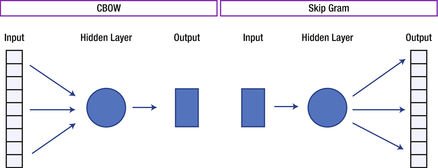
How It Works
The above figure shows the architecture of the CBOW and skip-gram algorithms used to build word embeddings. Let’s look at how these models work.
skip-gram
The skip-gram model 1 predicts the probabilities of a word given the context of the word or words.
Let’s take a small sentence and understand how it works. Each sentence generates a target word and context, which are the words nearby. The number of words to be considered around the target variable is called the window size. The following table shows all the possible target and context variables for window size 2. Window size needs to be selected based on data and the resources at your disposal. The larger the window size, the higher the computing power.
Target word | Context | |
|---|---|---|
I love NLP | I | love, NLP |
I love NLP and | love | love, NLP, and |
I love NLP and I will learn | NLP | I, love, and, I |
… | … | … |
in 2 months | month | in, 2 |
Since it takes a lot of text and computing power, let’s use sample data to build a skip-gram model.
We get an error saying the word doesn’t exist because this word was not in our input training data. We need to train the algorithm on as large a dataset as possible so that we do not miss words.
Continuous Bag of Words (CBOW)

Training these models requires a huge amount of computing power. Let’s use Google’s pre-trained model, which has been trained with more than 100 billion words.
Download the model from https://drive.google.com/file/d/0B7XkCwpI5KDYNlNUTTlSS21pQmM/edit and keep it in your local storage.
https://drive.google.com/file/d/0B7XkCwpI5KDYNlNUTTlSS21pQmM/edit
If you add woman and king and subtract man, it predicts queen as the output with 77% confidence. Isn’t this amazing?

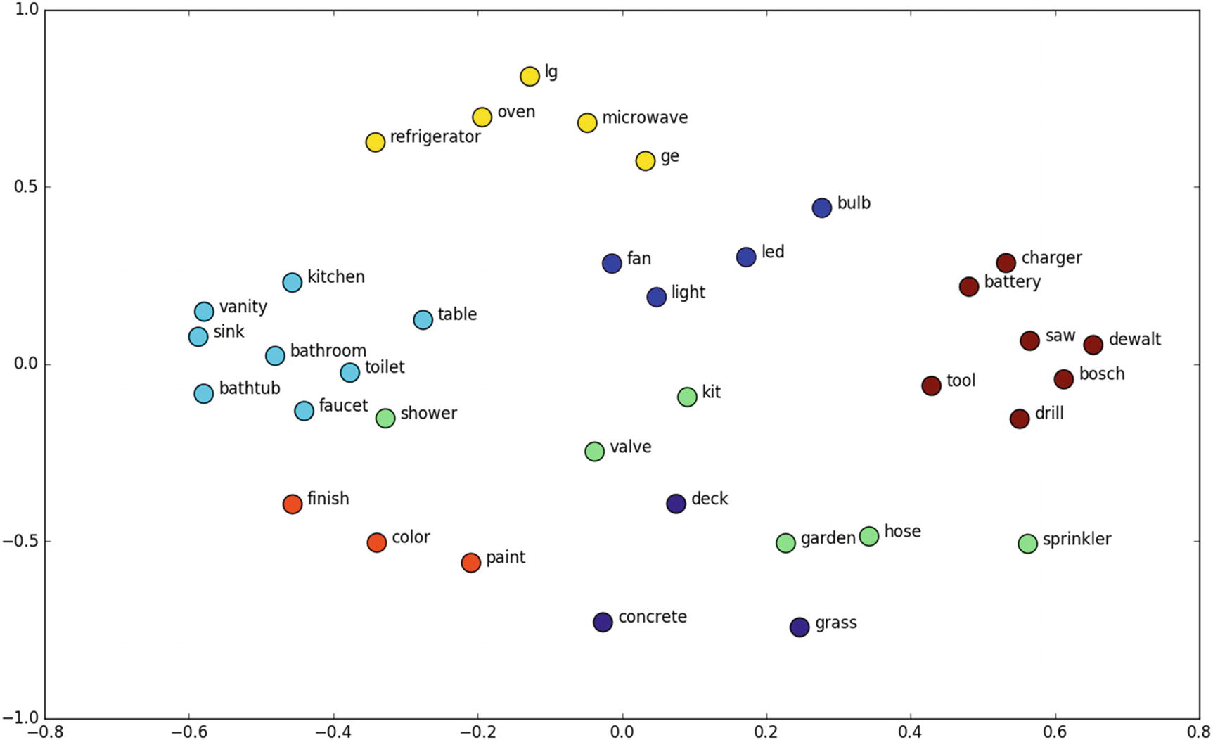
Let’s look at a few interesting examples using the t-SNE plot for word embeddings, such as for home interiors and exteriors. For example, all the words related to electrical fittings are near each other; similarly, words related to bathroom fittings are near each other, and so on. This is the beauty of word embeddings.
Recipe 3-8. Implementing fastText
fastText is another deep learning framework developed by Facebook to capture context and generate a feature vector.
Problem
You want to learn how to implement fastText in Python.
Solution
fastText is the improvised version of word2vec, which considers words to build the representation. But fastText takes each character while computing a word’s representation.
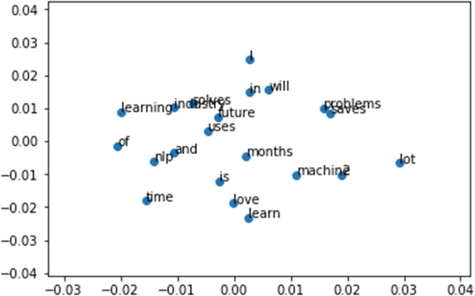
How It Works
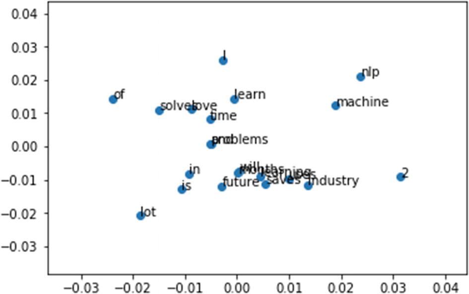
The figure above shows the embedding representation for fastText. If you observe closely, the words love and solve are close together in fastText but in your skip-gram and CBOW, love and learn are near to each other . This is because of character-level embeddings.
Recipe 3-9. Converting Text to Features Using State-of-the-Art Embeddings
Let’s discuss and implement some advanced context-based feature engineering methods.
Problem
You want to learn text to features using state-of-the-art embeddings.
Solution
GloVe Embedding
ELMo
- Sentence encoders
doc2vec
Sentence-BERT
Universal Encoder
InferSent
Open-AI GPT
GloVe is an alternate word embedding method to create vector subspace of the word. GloVe model trains on co-occurrence counts of words, and by minimizing least square error, it produces vector space.
In GloVe, you first construct co-occurrence: each row is a word, and each column is the context. This matrix calculates the frequency of words with context. Since the context dimension is very large, you want to reduce the context and learn a low-dimensional representation of word embedding. This process can be regarded as the reconstruction problem of the co-occurrence matrix, namely reconstruction loss. The motivation of GloVe is to explicitly force the model to learn such a relationship based on the co-occurrence matrix.
word2vec, skip-gram, and CBOW are predictive and ignore the fact that some context words occur more often than others. They only take into consideration the local context and hence failing to capture the global context.
While word2vec predicts the context of a given word, GloVe learns by constructing a co-occurrence matrix.
word2vec does not have global information embedded, while GloVe creates a global co-occurrence matrix counting frequency of context with each word. The presence of global information makes GloVe better.
GloVe does not learn by a neural network like word2vec. Instead, it has the simple loss function of the difference between the product of word embeddings and log of the probability of co-occurrence.
The research paper is at https://nlp.stanford.edu/pubs/glove.pdf.
ELMo
ELMo vectors are the vectors that are the function of a given sentence. The main advantage of this method is it can have different vectors of words under different contexts.
ELMo is a deep contextualized word representation model. It looks at complex characteristics of words (e.g., syntax and semantics), and studies how they vary across linguistic contexts (i.e., to model polysemy).
Word vectors are learned functions of the internal states of a deep bidirectional language model (biLM), which is pre-trained on a large text corpus.
Words with different contexts in different sentences are called polysemous words. ELMo can successfully handle words of this nature, which GloVe and fastText fail to capture.
The research paper is at www.aclweb.org/anthology/N18-1202.pdf.
Link to research paper: https://www.aclweb.org/anthology/N18-1202.pdf
Sentence Encoders
Why learned sentence embeddings? Traditional techniques use an average of the word embeddings to form sentence embeddings. But there are cons to this approach, such as the order of the words are not considered, and the similarities obtained by averaging word vectors are the same if the words are swapped in a sentence.
doc2vec
doc2vec is based on word2vec. Words maintain a grammatical structure, but documents don’t have any grammatical structures. To solve this problem, another vector (paragraph ID) is added to the word2vec model. This is the only difference between word2vec and doc2vec.
Distributed Memory Model of Paragraph Vectors (PV-DM)
Distributed Bag of Words version of Paragraph Vector (PV-DBOW)
The distributed memory (DM) model is similar to the CBOW model. CBOW predicts the target word given its context as an input, whereas in doc2vec, a paragraph ID is added.
The Distributed Bag-Of-Words (DBOW) model is similar to the skip-gram model in word2vec, which predicts the context words from a target word. This model only takes paragraph ID as input and predicts context from the vocabulary.
The research paper is at https://cs.stanford.edu/~quocle/paragraph_vector.pdf.
Sentence-BERT
Sentence-BERT (SBERT) is a modification of the pre-trained BERT network that uses siamese and triplet network structures to derive semantically meaningful sentence embeddings that can be compared using cosine-similarity. This reduces the effort of finding the most similar pair from 65 hours with BERT/RoBERTa to about 5 seconds with SBERT while maintaining the accuracy from BERT.
Attention
Transformers
BERT
Siamese networks
Sentences are passed to BERT models and a pooling layer to generate their embeddings.
The research paper is at www.aclweb.org/anthology/D19-1410.pdf.
Universal Encoder
The Universal Sentence Encoder model specifically targets transfer learning to the NLP tasks and generates embeddings.
It is trained on a variety of data sources to learn for a wide variety of tasks. The sources are Wikipedia, web news, web question-answer pages, and discussion forums. The input is variable-length English text, and the output is a 512-dimensional vector.
Sentence embeddings are calculated by averaging all the embeddings of the words in the sentence; however, just adding or averaging had limitations and was not suited for deriving the true semantic meaning of the sentence. The Universal Sentence Encoder makes getting sentence-level embeddings easy.
Transformers
Deep Average Network
The research paper is at https://arxiv.org/pdf/1803.11175v2.pdf.
InferSent
In 2017, Facebook introduced InferSent as a sentence representation model trained using the Stanford Natural Language Inference datasets (SNLI) . SNLI is a dataset of 570,000 English sentences, and each sentence is a pair sentence of the premise, hypothesis labeled in one of the following categories: entailment, contradiction, or neutral.
The research paper is at https://arxiv.org/pdf/1705.02364.pdf.
Open-AI GPT
The GPT (Generative Pre-trained Transformer ) architecture implements a deep neural network, specifically a transformer model, which uses attention in place of previous recurrence-based and convolution-based architectures. Attention mechanisms allow the model to selectively focus on segments of input text it predicts to be the most relevant.
Due to the broadness of the dataset on which it is trained and the broadness of its approach, GPT became capable of performing a diverse range of tasks beyond simple text generation: answering questions, summarizing, and even translating between languages in a variety of specific domains.
The research paper is at https://cdn.openai.com/better-language-models/language_models_are_unsupervised_multitask_learners.pdf.
How It Works
Download the dataset from www.kaggle.com/rounakbanik/ted-talks and keep it in your local folder. Then follow the steps in this section.
Dataset link: https://www.kaggle.com/rounakbanik/ted-talks
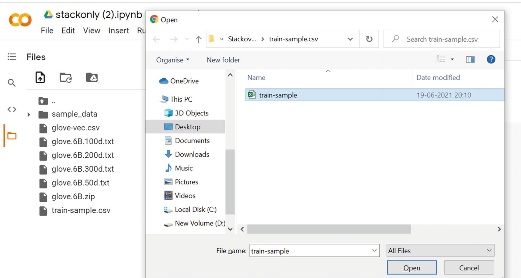
Step 9-1. Import a notebook and data to Google Colab
Google Colab is used to solve this project given BERT models are huge, and building it in Colab is way easier and faster.
Go to Google Colab at https://colab.research.google.com/notebooks/intro.ipynb.
https://colab.research.google.com/notebooks/intro.ipynb
Go to file and open a new notebook or Upload notebook from your local by selecting “Upload notebook”.

To import the data, go to Files, click the Upload to Session Storage option, and then import the csv file.
Step 9-2. Install and import libraries
Step 9-3. Read text data
Step 9-4. Process text data
Step 9-5. Generate a feature vector
Sentence-BERT
Universal Encoder
Infersent
Open-AI GPT
Step 9-6. Generate a feature vector function automatically using a selected embedding method
We hope that you are now comfortable with natural language processing. Now that the data has been cleaned and processed, and features have been created, let’s jump into building applications that solve business problems.