Chapter 2: Assembly Language

There are various types of programming languages, and in this chapter, we will focus on the low-level variant that is often known as an assembler language. The assembly language has a close relationship with the architecture's machine code instructions and is unique to that machine. As a result, many machines use distinct assembly languages. Symbols are used to represent an operation or command in this form of language. Therefore, it's also known as symbolic machine code.

Due to the reliance on machine code, assembly language is tailored to single computer architectures. You will find assembly language for architectures such as x86, x64, and ARM.

In this chapter, we will discuss the following topics:

• Demystifying assembly language
• Types of assembly language
• Identifying the elements of assembly language

Technical requirements

In this chapter, we will compile a simple script to view the assembly language. If you would like to replicate this in your own environment, you will need the following:

• A text editor (Nano, Vim, and so on)
• A GCC compiler
• Operating system used: Debian Linux

Demystifying assembly language

Assembly language (often abbreviated to asm) enables communication directly with the computer's processor. Since assembly language is a very low-level programming language, it is generally used for specific use cases, for example, writing drivers and shellcode. Trying to write a fully fledged program using assembly language would be near impossible, hence these are written with high-level languages.

Understanding assembly language helps you become aware of a number of things, especially in relation to the shellcode. For instance, you will be able to understand the following:

• The interaction between various components within a computer
• The representation of data in storage, in memory, and miscellaneous devices
• How instructions are accessed and executed by the processor
• How data is accessed and processed by instructions
• The manner in which a program interacts with external devices

Assembly language consists of the following:

• Executable instruction sets
• Assembler commands or pseudo-ops
• Macros

The processor is told what to perform by the instructions. An operation code is included in each instruction (opcode). One machine language instruction is generated for each executable instruction.

Assembler directives, sometimes known as pseudo-ops, provide information to the assembler that provides insight into the various steps of the assembly procedures. These procedures aren't executable and don't generate machine language commands.

Macros are a type of text replacement technique.

Assembly language statements are entered per line. It follows the format of [label] mnemonic [operands] [;comment]. An example of this is as follows:

mov RX, 13  ; Transfer the value 13 to the RX register

Each low-level machine instruction or opcode, as well as each architectural register, flag, and so on, is represented by a mnemonic in assembly language. Each statement in assembly language is broken down into an opcode and an operand. The opcode is the instruction that the CPU executes, and the operand is the data or memory location where that instruction is performed.

For example, let's consider the following line of assembly:

mov    ecx,  msg

The opcode used here is mov, ecx (register), and msg. These are all operands and this assembly instruction is moving a message to the ecx register.

Assembly language makes use of instructions that work directly with a processor. The purpose of these instructions is to tell the processor how to work with its components. For example, it will provide an instruction to move specific data from a register to a program's stack or move a value to a register, and so forth.

In the previous chapter, the examples you have seen were written with a high-level language. When a high-level language is used, you define the variables, and the compiler takes care of the internals. Let's take a look at a sample of Hello World written in C:

#include <stdio.h>

char s[] = "Hello World";

int main ()

{

    int x = 2000, z =21;

    printf("%s %d /n", s, x+z);

}

You can run this in your own Kali environment by adding the preceding text to a file.

Next, you will save this file to hello.c. Then you will use a compiler called GCC to compile this into assembly language, using the following command:

gcc –S hello.c

Note

When you use the GCC compiler, the normal flow would be to compile and link the code to create an executable. Using the –S command will stop the process after compilation, allowing you to see the assembly code. You will get output in the form of assembly code. The source file extension will change from .c to .s.

Let's examine the hello.s file to view the assembly language for the script we have just created. The assembly code contains various instructions as per the following example:

.file "hello.c"

.text

.globl s

.data

.align 8

.type s, @object

.size s, 13

s:

.string "Hello World"

.section .rodata

.LC0:

.string "%s %d "

.text

.globl main

.type main, @function

main:

.LFB0:

.cfi_startproc

Pushq %rbp

.cfi_def_cfa_offset 16

.cfi_offset 6, -16

Movq %rsp, %rbp

.cfi_def_cfa_register 6

Subq $16, %rsp

Movl $2000, -4(%rbp)

Movl $21, -8(%rbp)

Movl -4(%rbp), %edx

Movl -8(%rbp), %eax

Addl %edx, %eax

Movl %eax, %edx

Leaq s(%rip), %rsi

Leaq .LC0(%rip), %rdi

Movl $0, %eax

Call printf@PLT

Movl $0, %eax

leave

.cfi_def_cfa 7, 8

ret

.cfi_endproc

As you can see, if you had to fully compile this piece of code and run it, the result would be the text Hello World 2021 presented on the screen.

In the preceding assembly code, each line corresponds to a machine instruction. You will notice the mnemonic opcodes, registers, and operands being used. For example, you can see movl being used since we used an integer in the code. You will notice the various registers being called (edx, eax, and so on) and the printf system call. This output aims to introduce you to the assembly language and how it is depicted. As you work through the chapter, you will understand the various registers, instructions, and their uses.

Types of assembly language

A microprocessor performs various functions. These functions span arithmetic calculations, logic operations, and control functions. Each processor family has its own instruction sets that are used for handling various tasks. These tasks range from keyboard inputs, displaying information on a screen, and more. Remember that machine language instructions, which are binary strings of 1s and 0s, are all that a processor understands. Machine language is far too opaque and sophisticated to be used in the development of day-to-day software. As a result, the low-level assembly language is tailored to a certain processor generation and encodes various instructions in symbolic code in a more intelligible manner.

Assembly language architecture spans x86, x64, ARM assembly, and more.

Identifying the elements of assembly language

As you work with shellcode and start seeing it visualized in assembly language, you will notice that an assembly program can be divided into three sections:

• The data section declares initialized data. At runtime, this data remains unchanged. In this area, you will find various constant values, filenames, buffer sizes, and so forth. The data section starts with the section.data declaration.
• The bss section is used to declare variables; this is depicted by section.bss.
• The text section is where the actual code or instructions are kept. This is depicted by section.text and begins with a global_start declaration that informs the kernel of the execution point of the program. The code sequence for this text section looks as follows:

  section.text   

  global _start

  _start:

When you work with assembly language, it's important to understand the various elements that you will find within it. Recall the example at the beginning of this chapter. Once the hello.c file was compiled, the resulting assembly code contained a number of opcodes, registers, and operands. In this section, we will cover those various components. Further research on assembly language is encouraged since covering all of the various registers, instructions, and so on would far exceed the aim of this book.

Registers and flags

In computing architecture, the central processing unit (CPU) is responsible for the processing of data. So, let's take a step back and visualize a computer in simple building blocks. The following figure focuses on just three basic components of a computer system:

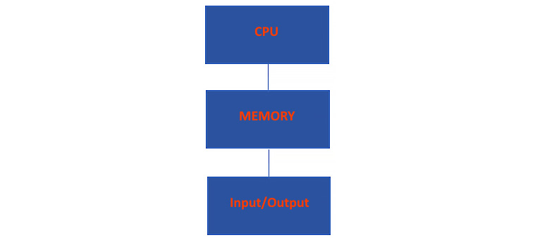
Figure 2.1 – Components of a computer system

The three simplest components are CPU, memory, and I/O. The CPU, being the brains of everything, needs to execute data. So, let's take a look at the components specifically related to the CPU and what their uses are.

We will begin with the control unit. The control unit is responsible for directing the computer's memory, arithmetic logic unit, and various I/O devices on how to respond to instructions that have been received by the CPU. It will also fetch instructions from various locations, such as memory and registers, and ultimately supervise the execution of them.

The next component is the execution unit. This component is where the actual execution of instructions happens.

The next two components are registers and flags. We will focus on registers and flags in depth later in this chapter.

Now that we have a high-level overview of the architecture of a CPU, let's focus on how it stores and executes data. This data can either be stored in registers or memory locations. One of the main differences between registers and memory locations is the access time. Since registers are closer to the processor, the access time is very fast. To illustrate the difference in speed, consider really fast RAM chips. These would have an access time of around 10-50 nanoseconds, whereas accessing a register would be around 1 nanosecond.

The following table illustrates the speed of registers in comparison to other types of storage.

Figure 2.2 – Access speed comparison

Registers form the smallest component of memory, and although it's the smallest, it's the fastest. Data stored in registers is not persistent. Next, you have the CPU cache, which can hold more than a register and is used by CPUs to reduce the average time it takes to access data. Registers and the cache are high speed, and they are placed between the CPU and RAM to improve speed and performance. RAM has a much higher capacity, and as advancements are made with respect to the speed of RAM, it is still not as fast as a cache or register. Finally, you have the largest, slowest, and most inexpensive hard drives or solid-state drives. They offer large storage and relatively quick read and write times, but not as quick as RAM, cache, or registers.

Let's provide an overview of the various types of registers.

General-purpose register

We begin with general-purpose registers (GPR). They are used to store data temporarily in the CPU. There are 16 GPRs, each of which is 64 bits long. GPRs are outlined in Figure 2.2. A GPR can be accessed using all 64 bits or just a subset of them.

Note

64-bit registers start with an r, whereas 32-bit registers start with an e. Throughout this book, we will refer to various 64-bit and 32-bit registers. It would be good to keep this table handy:

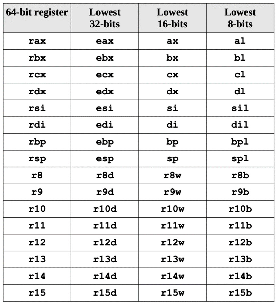
Figure 2.3 – Breakdown of common registers

In the given table, you will find a quick reference to a number of registers that span various architectures. Let's focus on the 16-bit registers and break down their uses:

• AX: The accumulator is designated by AX. This register consists of 16 bits, which is further split into registers such as AH and AL, which are 8 bits each. This split enables the AX register to process 8-bit instructions as well. You will find this register involved in arithmetic and logic operations.
• BX: The base register is designated by BX. This 16-bit register is also split into two 8-bit registers, which are BH and BL. The BX register is leveraged to keep track of an offset value.
• CX: The counter register is designated by CX. CX is split into CH and CL, which are 8 bits each. This register is involved in the looping and rotation of data.
• DX: The data register is designated by DX. This register also contains two 8-bit registers, which are DH and DL. The function of this register is to address input and output functions.

When employing data element sizes smaller than 64 bits (32-bit, 16-bit, or 8-bit), the lower section of the register can be accessed by using a different register name, as shown in Figure 2.2. To illustrate, let's look at the rax register. Figure 2.3 details the layout for accessing the lower portions of the 64-bit rax register:

Figure 2.4 – Breakdown of the RAX register, including 32-bit and 16-bit registers

The first four registers, rax, rbx, rcx, and rdx, give access to bits 8–15 using the ah, bh, ch, and dh register names, as indicated in Figure 2.3 and Figure 2.4. These are given for legacy support, with the exception of ah.

Viewing registers of bin/bash

Now, I am fully aware that reading all of this may be a lot to take in, so let's look at this with the help of an example. I will use the GNU Project Debugger program on my Kali Linux machine to debug /bin/bash on my computer:

Note

If you do not have the GNU Debugger installed, this can be done using the following command: sudo apt install gdb.

1. Since my Kali Linux machine is x64, we will see the 64-bit registers and be able to view their 32-bit components as well. I will issue the command to start the debugger, which is as follows:

   gdb /bin/bash

2. Next, I will define a breakpoint so that the program will stop at the main function. This is done by issuing the following command:

   break main

3. Next, I will run the program using the following command:

   run

Now the debugger will stop at the breakpoint on the main section. This is depicted in the following screenshot:

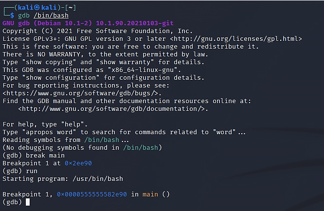
Figure 2.5 – Debugging of /bin/bash with gdb

4. Now that we have hit the breakpoint, let's look at the registers by issuing the following command:

   info registers

You will now be able to view the registers as shown in the following screenshot. Please note that the address values would be different on your system.

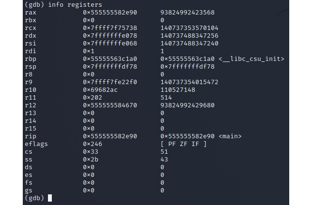
Figure 2.6 – Registers in use by /bin/bash/

Let's focus on the RAX register. If you revisit Figure 2.3 and Figure 2.4, you will see that the RAX 64-bit register contains the EAX 32-bit register. Within that EAX register, you will find AX, which is 16 bits, and finally, within that, you will find the registers of AH and AL, which are 8 bits.

5. You can view this in gdb. Let's look at the value of EAX by running the following command:

   display /x $eax

In my system, the returned value is 1: /x $eax = 0x55582e90. This is the 32-bit value of my RAX register, which we can see in Figure 2.6.

6. To view the value of the AX register, you can run the preceding command, but this time using the value of ax, as follows:

   display /x $ax

This will give you the value of the 16-bit register. You can use the same command to drill down to the AL register. The following screenshot shows the values within my system:

Figure 2.7 – Breaking down the RAX register

This exercise can also be performed on the other registers to help you visualize how the registers are broken down. Now, let's move on to the next section, which concerns pointer registers.

Pointer register

A pointer register is a register used to store a memory address in the computer processor architecture. You might be able to use it for other things as well, but they are usually instructions that interpret it as a memory address and retrieve the data stored at that address. Let's look at some of the pointer registers and their functions:

• SP: This stands for stack pointer. It has a bit size of 16 bits. It indicates the stack's highest item. The stack pointer will be (FFFEH) if the stack is empty. It's a relative offset address to the stack section.
• BP: The base pointer is denoted by the letters BP. It has a bit size of 16 bits. It is mostly used to access stack-passed arguments. It's a relative offset address to the stack section.
• IP: This determines the address of the next instruction that will be executed. The whole address of the current instruction in the code segment is given by IP in conjunction with the code segment (CS) register as (CS: IP).

  Note

  The CS register is used when addressing the memory's code segment or the location where the code is stored. The offset within the memory's code section is stored in the instruction pointer (IP).

Index registers

The current offset of a memory location is stored in an index register, and the base address is stored in another register, resulting in a completed memory address. For example, in Figure 2.8, you will see that the 32-bit index registers, comprising ESI and EDI, and their 16-bit counterparts, SI and DI, are used for indexed addressing. These registers are sometimes used in arithmetic functions such as addition and subtraction.

Figure 2.8 – Breakdown of index registers

The two types of index registers are as follows:

• Source Index (SI): This is the register for the source index. It has a bit size of 16 bits. It's utilized for data pointer addressing and as a source for various string operations. It has a relative offset to the data segment.
• Destination Index (DI): This is the register used for the destination index.

Now that we have covered index registers, let's move on to control registers.

Control registers

Control registers come into play when instructions make use of comparisons and mathematical operations to change the status of flags, while others use conditional instructions to test the value of these status flags before diverting the control flow to another place. When you combine pointer registers and flag registers, these are considered control registers.

The most common flags that work with control registers are:

• Overflow Flag (OF): Once a signed arithmetic operation completes, it signifies the overflow of a higher-order bit (which will be the leftmost bit) of data.
• Direction Flag (DF): This determines whether to move or compare string data in the left or right direction. When the DF value is 0, the string operation is performed left to right, and when the value is 1, the string operation is performed right to left.
• Interrupt Flag (IF): This specifies whether external interrupts, such as the input of a keyboard, should be ignored or processed. When set to 0, it inhibits external interrupts, and when set to 1, it enables them.
• Trap Flag (TF): This allows you to set the CPU to operate in single-step mode. The TF is set by the DEBUG program, which allows us to walk through the execution. This walk-through is executed as per instructions.
• Sign Flag (SF): This displays the sign of the result of an arithmetic operation. Following an arithmetic operation, this flag is set based on the sign of the data item. The most significant bit of the leftmost bit indicates the sign. A positive result resets the SF value to 0, and a negative result resets it to 1.
• Zero Flag (ZF): This denotes the outcome of a calculation or a comparison. When a result is equal to non-zero, this will result in the ZF being set to 0; conversely, when a result is zero, then the ZF will be set to 1.
• Auxiliary Carry Flag (AF): When it comes to binary coded decimal operations, or BCD as it is abbreviated, the auxiliary carry flag would come into play. It is related to math operations and is set when there is a carry from a lower bit to a higher bit, for example, from bit 3 to bit 4.
• Parity Flag (PF): When an arithmetic operation takes place and the resulting bits are even, then the parity flag gets set. If the result is not even, the parity flag will be set to 0.
• Carry Flag (CF): Upon completion of an arithmetic operation, the CF reflects the carry of 0 or 1 from a high-order bit (leftmost). It also saves the contents of a shift or rotates the operation's last bit.

Next, we need to understand how memory locations are handled in assembly language. This is where segment registers come into play.

Segment registers

Inside the CPU, segment registers are basically memory pointers. Segment registers point to a memory location where one of the following events takes place: data location, an instruction to be executed, and so on.

When it comes to segment registers, let's focus on the following:

• Code Segment: This covers all of the directions that must be carried out. The CS register is used to store the starting address of the code segment.
• Data Segment: Data, constants, and work areas are all included. The DS register is used to store the starting address of the data segment.
• Stack Segment: This contains information on procedures and subroutines, as well as their return addresses. The implementation of this is in the form of a data structure known as a stack. The stack's starting address is stored in the stack segment register, or SS register.

The segment's start address is stored in the segment register. The offset value (or offset) is needed to find the exact location of data or instructions in a segment. The processor refers to the memory location of the segment by associating the segment address in the segment register with the location offset value.

Data movement instructions

Data movement instructions transfer information from one area to another, which is referred to as the source and destination operands. Loads, stores, moves, and immediate loads are several types of data movement instructions.

Data movement instructions can be inserted in the following categories:

• Instructions that are used for general purposes
• Instructions related to the manipulation of the stack
• Instructions related to type conversions

General-purpose movement instructions

During the program flow, data would need to be moved around. For example, you may need to move a register or move data between memory locations, and so forth. This is where general-purpose movement instructions are used. Let's take a look at the following general-purpose instructions – MOV, MOVS, and XCHG:

• MOV: This is a command that moves data from one operand to another. This data can be in the form of a byte, word, or even a double word. Any of these pathways can be used with the MOV instruction to transfer data. There are also MOV variations that work with segment registers.

This instruction does not provide the capability to move from one memory location to another or from a segment register to another. The move string instruction MOVS, on the other hand, can conduct memory-to-memory movements.

• MOVS: Since the MOV instruction is not able to provide the capability to move data from one memory location to another, or from a segment register to another, the MOVS instruction fulfills this purpose, as it can also be used to move strings one byte at a time.

Here are some examples of MOV instructions:

• mov eax, 0xaaabbbcc: This moves data to the EAX register.
• mov rbp, rax: This moves data between registers.

• XCHG: This exchanges two operands' contents. Three MOV instructions are replaced by this instruction. It is not necessary to save the contents of one operand while the other is being loaded in a temporary place. XCHG is particularly handy for implementing semaphores or other synchronization data structures.

This exchange instruction can be used to swap operands; for example, it can be used to swap a memory address with an AX register. XCHG automatically activates the LOCK signal when used with a memory operand.

Next, we will look at the instructions that can be used for stack manipulation.

Stack manipulation instructions

To directly alter the stack, stack manipulation instructions are utilized.

• POP: This transfers a value that is currently at the top of the stack to a destination operand. Once this is done, the ESP register is incremented to point to the new stack value. POP can also be used with segment registers.
• POPA: POPA means to pop all registers. This instruction is used to restore the general-purpose registers. POPA on its own is a 16-bit register. This means that the first register to be popped would be DI, followed by SI, BP, BX, DX, CX, and AX. POPAD, on the other hand, is a 32-bit register. Essentially, POPAD is referring to a double word, so in this case, the first register to be popped would be EDI, followed by ESI, EBP, EBX, EDX, ECX, and EAX.
• PUSHA: PUSHA, which means push all registers, saves the contents of the stacks registers. The POPA instruction is used in conjunction with PUSHA, and the same applies to PUSHAD in relation to POPAD.
• PUSH: PUSH is commonly used to store parameters on the stack; it is also the primary method of storing temporary variables on the stack. Memory operands, immediate operands, and register operands are all affected by the PUSH instruction (including segment registers).

As we conclude this section, it may seem like a lot to take in. However, once we start working with shellcode and viewing programs in a disassembler, all of these instructions will become clearer. Now let's move on to arithmetic instructions.

Arithmetic instructions

Within a CPU, you will find a component that is called the Arithmetic Logical Unit (ALU). This component is responsible for performing arithmetic operations such as addition, subtraction, and multiplication.

In assembly language, these operations are depicted as follows:

• Addition (add)
• Subtraction (sub)
• Division (div)
• Multiplication (mul)

Arithmetic instructions follow the same syntax as assembly language, as we have seen previously:

operation destination, source

The syntax is explained here:

• operation refers to the intended arithmetic operation (add, sub, div, mul).
• destination refers to the memory location or register where the final result will be stored once the operation is completed.
• source refers to the memory location or register that contains the initial value on which the operation will act.

  Note

  There are differences in the way AT&T and Intel assembly language is written. You can view this write-up at the following link: http://staffwww.fullcoll.edu/aclifton/courses/cs241/syntax.html.

For example, let's examine the following piece of code, which performs the various arithmetic instructions on the values defined by a and b:

#!/bin/sh

a=100

b=50

val='expr $a + $b'  #Line 1

echo "a + b : $val" #Line 2

val='expr $a - $b'  #Line 4

echo "a - b : $val" #Line 5

val='expr $a * $b'  #Line 7

echo "a * b : $val"  #Line 8

val='expr $a / $b'  #Line 10

echo "b / a : $val"  #Line 11

On line 1, we have the addition operation being performed on the two values declared by a and b. The result here would produce a value of 150. Line 4 performs a subtraction operation on the values, returning the result of 50. Line 7 performs multiplication on the values, returning the result of 5000. Lastly, line 10 performs division on the values, resulting in 2.

Arithmetic instructions are often used in shellcode. As we work through the chapters related to Linux and Windows shellcode, you will find arithmetic instructions across the various samples of shellcode.

Conditional instructions

Conditional instructions within assembly language can be used to change the way a program operates. These changes to the flow of the program are usually done during its runtime by making branches (jumps) or executing certain instructions only when a condition is met.

The common types of conditional instructions that you will come across are conditional jumps and unconditional jumps. Let's take a look at what each of these instructions entails.

Conditional jump

Conditional jumps are used to make decisions based on the status flags' values or a condition. When notions such as if statements and loops must be employed in Assembly, conditional jumps are typically used. Conditional jumps are used to determine whether or not to take a jump because assembly language does not support words such as if statements.

Depending on the condition and data, there are a variety of conditional jump instructions. For example, the following table depicts the conditional jump instructions used on signed data that is used for arithmetic operations.

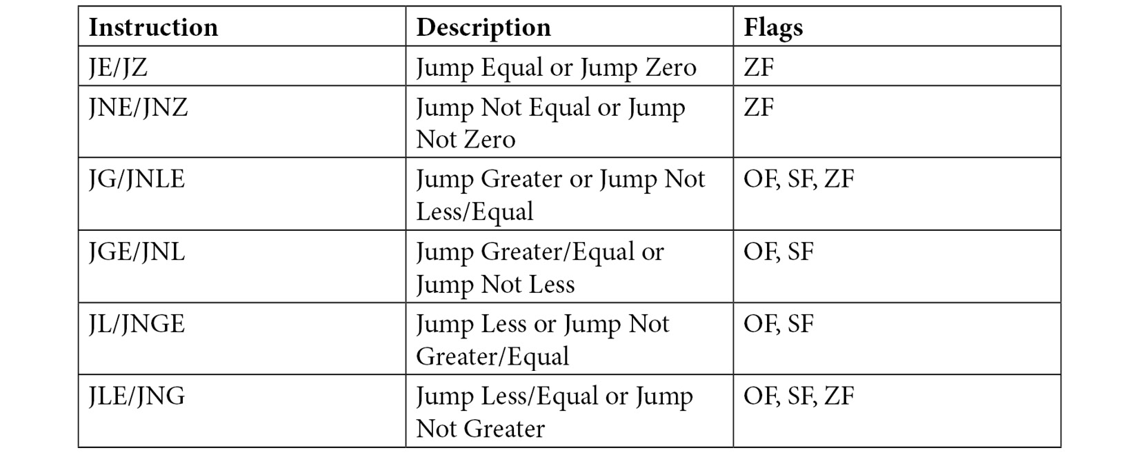
Table 2.1 – Jump instructions broken down. Source: https://www.tutorialspoint.com/assembly_programming/assembly_conditions.htm

Note

The flags depicted here represent the zero flag (ZF), overflow flag (OF), and sign flag (SF). These flags are part of the x86 architecture.

There are conditional instructions that relate to logical operations and some that have a special use case. Detailing them far exceeds the scope of this book, but you can find information about this in the Intel architecture manual found in the Further reading section of this chapter. For now, it's important to note that conditional jump instructions exist, and that these can be used in shellcode.

Unconditional jump

An unconditional jump works whereby a program jumps to a label that is defined in the instruction. These unconditional jumps are essentially broken down into three types – short jump, near jump, and far jump:

• A short jump is a 2-byte instruction that allows access or jumps to memory locations that are defined within a certain memory byte range. This memory byte range is 127 bytes ahead of the jump or 128 bytes behind the jump instruction.
• A near jump is a 3-byte jump that allows access to +/- 32K bytes from the jump instruction.
• A far jump works with a specified code segment. In the case of a far jump, the value is absolute, meaning that the instruction will jump to a defined instruction.

Conditional instructions, especially the various jumps, can be used when you want to jump to your shellcode. If you have control of an instruction pointer and your shellcode resides therein, a jump can be used to reference that pointer. If you take a simple buffer overflow example, by incorporating either an unconditional or conditional jump in an exploit, you essentially hop to different sections of the buffer to reach the shellcode.

Summary

In this chapter, we looked at how the computer works at a lower level than C code: it performs a series of assembly instructions, which are simple actions that convert into processor circuit operations. Assembly is difficult to write but being able to understand it intuitively is useful. So, we covered a lot of material regarding assembly language, and further study is encouraged since assembly language is such a large topic.

We learned that there are calculation, data movement, and control flow instructions in assembly and that the compiler frequently generates unexpected instruction sequences to speed things up. This is one of the reasons we use compilers: they are good at condensing our programs into the shortest possible sequence of instructions.

In the next chapter, we will focus a bit more on assembly language and then we will move on to compilers, tools for shellcode, and more.

Further reading

• Intel 64 and IA-32 Software Developers Manual: https://www.intel.com/content/dam/www/public/us/en/documents/manuals/64-ia-32-architectures-software-developer-instruction-set-reference-manual-325383.pdf.