Why is everybody still using JPEG files if they can only distinguish between 255 different levels? Does it mean it can only capture a dynamic range of 1:255? It turns out there are clever tricks that people use.

As we mentioned before, the camera sensors capture values that are linear, that is, 4 means that it has 4 times more light than 1, and 80 has 8 times more light than 10. But does the JPEG file format have to use a linear scale? It turns out that it doesn't. So, if we are willing to sacrifice the difference between two values, for example, 100 and 101, we can fit another value there.

To understand this better, let's look at the histogram of gray pixel values of a RAW image. Here is the code to generate that—just load the image, convert it to grayscale, and show the histogram using pyplot:

    images = [load_14bit_gray(p) for p in args.images]
    fig, axes = plt.subplots(2, len(images), sharey=False)
    for i, gray in enumerate(images):
        axes[0, i].imshow(gray, cmap='gray', vmax=2**14)
        axes[1, i].hist(gray.flatten(), bins=256)

Here is the result of the histogram:

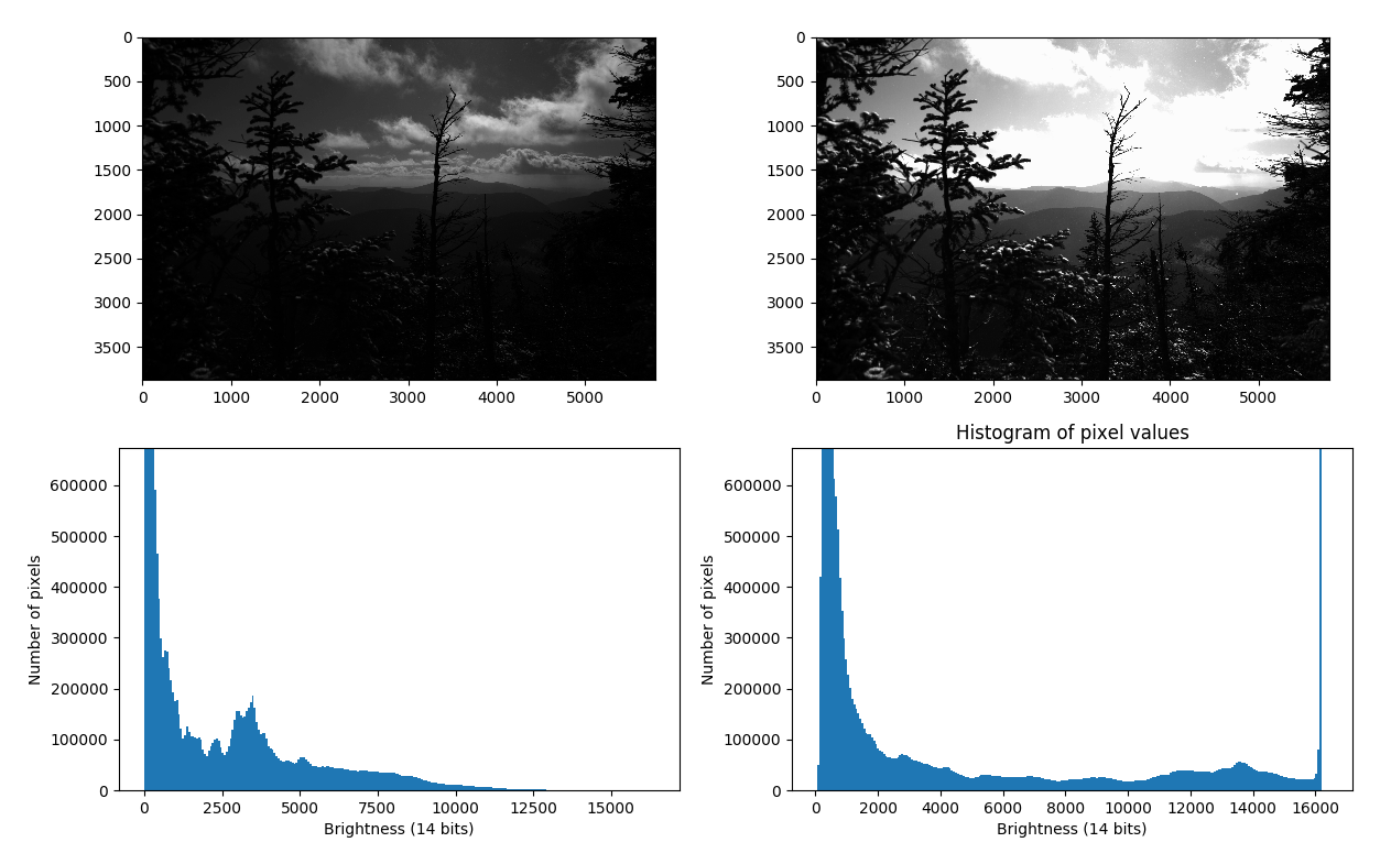
We have two pictures: the left one is a normal picture, where you can see some clouds, but it's almost impossible to see anything in the foreground, and the right one has tried to capture some detail in the trees, and because of that has burned all the clouds. Is there a way to combine these?

If we take a closer look at the histograms, we see that the burned-out part is visible on the right-hand histogram because there are values that are 16,000 that get encoded as 255, that is, white pixels. But on the left-hand picture, there are no white pixels. The way we encode 14-bit values into 8-bit values is very rudimentary: we just divide the values by 64 (=2⁶), so we lose the distinction between 2,500 and 2,501 and 2,502; instead, we only have 39 (out of 255) because the values in the 8-bit format have to be integers.

This is where gamma corrections come in. Instead of simply showing the recorded value as the intensity, we are going to make some corrections, to make the image more visually appealing.

We are going to use a non-linear function to try to emphasize the parts that we think are more important:

Let's try to visualize this formula for two different values—γ = 0.3 and γ = 3:

As you can see, small gammas put an emphasis on lower values; the pixel values from 0-50 are mapped to pixel values from 0-150 (more than half of the available values). The reverse is true of the higher gammas—the values from 200-250 are mapped to the values 100-250 (more than half of the available values). So, if you want to make your photo brighter, you should pick a gamma value of γ < 1, which is often called gamma compression. And if you want to make your photos dimmer to show more detail, you should pick a gamma value of γ > 1, which is called gamma expansion.

Instead of using integers for I, we can start with a float number and get to O, then convert that number to an integer to lose even less of information. Let's write some Python code to implement gamma correction:

1. First, let's write a function to apply our formula. Because we are using 14-bit numbers, we will have to change it to the following:

Thus, the relevant code will be as follows:

@functools.lru_cache(maxsize=None)
def gamma_transform(x, gamma, bps=14):
    return np.clip(pow(x / 2**bps, gamma) * 255.0, 0, 255)

Here, we have used the @functools.lru_cache decorator to make sure we don't compute anything twice.

2. Then, we just iterate over all the pixels and apply our transformation function:

def apply_gamma(img, gamma, bps=14):
    corrected = img.copy()
    for i, j in itertools.product(range(corrected.shape[0]),
                                  range(corrected.shape[1])):
        corrected[i, j] = gamma_transform(corrected[i, j], gamma, bps=bps)
    return corrected

Now let's take a look at how to use this to show the new image alongside the regularly transformed 8-bit image. We will write a script for this:

1. First, let's configure a parser to load an image and allow setting the gamma value:

 if __name__ == '__main__':
    parser = argparse.ArgumentParser()
    parser.add_argument('raw_image', type=Path,
                        help='Location of a .CR2 file.')
    parser.add_argument('--gamma', type=float, default=0.3)
    args = parser.parse_args()

2. Load the gray image as a 14bit image:

    gray = load_14bit_gray(args.raw_image)

3. Use linear transformation to get output values as an integer in the range [0-255]:

    normal = np.clip(gray / 64, 0, 255).astype(np.uint8)

4. Use our apply_gamma function we wrote previously to get a gamma-corrected image:

    corrected = apply_gamma(gray, args.gamma)

5. Then, plot both of the images together with their histogram:

    fig, axes = plt.subplots(2, 2, sharey=False)
    for i, img in enumerate([normal, corrected]):
        axes[0, i].imshow(img, cmap='gray', vmax=255)
        axes[1, i].hist(img.flatten(), bins=256)

6. Finally, show the image:

    plt.show()

We have now plotted the histogram and will look at the magic that is elaborated in the following two images with their histograms:

Look at the picture at the top right—you can see almost everything! And we are only getting started.

It turns out gamma compensation works great on black and white images, but it can't do everything! It can either correct brightness and we lose most of the color information, or it can correct color information and we lose the brightness information. So, we have to find a new best friend—that is, HDRI.