
Among programming techniques used for trading equity markets, Monte Carlo simulation has a special place due to factors such as its wide applicability and easy implementation. These methods can be used to implement strategies for market analysis such as price forecasting, or to validate options trading strategies, for example.
A great advantage of the Monte Carlo methods is the fact that they can be used to study complex events without the need to solve complicated mathematical models and equations. Using the idea of simulation through the use of random numbers, Monte Carlo methods offer the ability to study a large class of events, which would otherwise be difficult to analyze using exact techniques.
Random number generation: Generating random numbers is a basic step in creating algorithms that exploit stochastic behavior. Monte Carlo methods require the use of effective random number generation routines, which will be discussed in this chapter.
Probability distributions: Monte Carlo algorithms are based on the properties of stochastic events. Many of these events occur according to well-known probability distributions. In C++, it is possible to generate numbers according to many popular probability distributions, as you will learn.
Random walks: A random walk is a stochastic process where a certain quantity can randomly change with equal probability to positive or negative side. This makes random walk very useful for modeling prices in financial markets, as well as for simulating trading strategies.
Stochastic models for options pricing: Another application of random walks is in the determination of option prices. Using a stochastic method for this purpose is useful if you want to avoid the use of a more complex exact or approximate model, such as the algorithms described in the previous chapter.
Introduction to Monte Carlo Methods
A Monte Carlo algorithm is a computational procedure that uses random numbers to simulate and study complex events. It is based on the idea that you can analyze the results of an event by repeating it several times in different ways, with the help of a computer or other technique to generate random numbers.
This idea behind Monte Carlo methods is not new, having been used for as long as probability methods have been studied. For example, a well-known randomized procedure to determine the area of a geometric shape is to throw darts at the figure. After a while, you can count the percentage of darts inside the shape and use that percentage to determine the area.
Despite their simplicity, Monte Carlo methods may be time-consuming, and they require a large number of repetitions to achieve their goals. The recent development of fast computers, however, made it possible to use such methods in an increasing number of situations, making them practical and capable of finding solutions for problems where explicit mathematical analysis is very difficult.
Options pricing: It is possible to use randomized algorithms to determine the prices of options and other derivatives.
Trade strategy analysis: Monte Carlo methods can be used to test different trade strategies using simulated prices. This type of analysis is invaluable, since it allows you to test trading techniques on a large amount of data that is independent of the existing market observations.
Analysis of bonds and other fixed income investments: Bonds and their derivatives are tied to fluctuations of interest rates over different time horizons. An effective way to study the behavior of bonds is to construct stochastic models and use them to perform an analysis.
Portfolio analysis: Another area where Monte Carlo methods are useful is when studying a portfolio of investments. The stochastic algorithm allows analysts to vary the rate of exposure to diverse economic scenarios and try to determine the best allocation for a portfolio.
In the next few sections, you will first learn the tools necessary to design and implement Monte Carlo algorithms using the C++ language. You will also see examples of how these tools can be used to analyze options and related instruments.
Random Number Generation
The first topic that is addressed is random number generation. True random numbers are not possible to achieve in digital computers, but there are several techniques to create sequences of pseudo-random numbers. These methods have been made available through the standard C++ libraries, as will be covered in this section.
For C++ programmers, the main source of random number generation routines is the <random> header file provided by the standard library. With these functions, you can generate pseudo-random numbers that are well tested and that can be accessed through an easy interface.
Mersenne twister: This is one of the most popular generators. It is based on an algorithm that uses Mersenne prime numbers as the period length of the sequence of pseudo-random numbers. The Mersenne twister algorithm is considered to be one of the best general-purpose generators of random numbers, and it is frequently used in applications.
Linear congruential engine: This engine is based on a traditional algorithm that uses simple addition, multiplication, and module operations to produce numbers that have pseudo-random properties. This generator is indicated when you need fast sequences of random numbers, due to its efficiency. However, the linear congruential algorithm is known to generate numbers that possess some correlation.
Subtract with carry: This is still another algorithm that is used to generate random numbers in the standard library. The algorithm is called lagged Fibonacci, and it uses a numeric sequence that has properties that are similar to the famous Fibonacci sequence.
Algorithm for Pseudo-random Number Generation
Algorithm | Description |
|---|---|
Linear congruential | Traditional method that uses modulo arithmetic. |
Inversive congruential | Uses the modular multiplicative inverse to generate new elements in the sequence. |
Mersenne twister | Method developed in 1997; uses Mersenne primes to generate random numbers. |
WELL generators | Well Equidistributed Long-Period Linear, based on the application for operations on a binary field. |
XorShift generators | Fast method that uses exclusive-or operations to generate new random numbers. |
Linear feedback shift | Method that uses a linear function over the existing sequence of values to generate the next random number. |
Park-Miller generator | A linear congruential generator that uses multiplicative groups of integers under the modulo operation. |
A List of Generator Instantiations Available on the Standard Library
Generator Instantiation | Parameters |
|---|---|
default_random_engine | Random engine that is provided as a default option by the library implementation. |
knuth_b | Defined as typedef shuffle_order_engine <minstd_rand0,256> knuth_b;. |
minstd_rand | Minimal standard generator; it is an instantiation of linear_congruential_engine. |
minstd_rand0 | Similar to the engine described previously, with particular parameters. |
mt19937 | Mersenne twister generator. |
mt19937_64 | Mersenne twister generator for 64-bit types. |
ranlux24 | Uses the subtract-with-carry generator and returns values that use a 24-bit representation. |
Random number generators can be freely instantiated in the standard library. However, you should rarely need to define a new instantiation, unless you have good knowledge about how the parameters for each generator work together. A careful study of parameters is usually necessary to create a new generator, since they are based on statistical properties that have been determined after careful analysis made by researchers in the area.
The generators and their instantiations can be thought of as the original source for pseudo-random bits. Once you have defined a source, it is possible to generate random numbers according to a given probability distribution, as you will see in the next section.
Probability Distributions
A probability distribution is family of functions that defines the parameters for a stochastic process. For example, the simplest distribution of random numbers is the uniform distribution, where each value is generated with equal probability in a given range. A particular case of the uniform distribution is Uniform[0,1], where each number is randomly generated with equal probability in the range between 0 and 1.
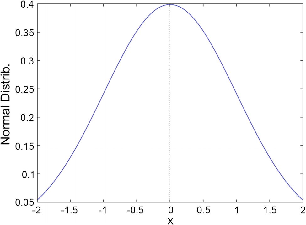
Probabilities defined by the normal distribution, with mean 0 and standard deviation 1
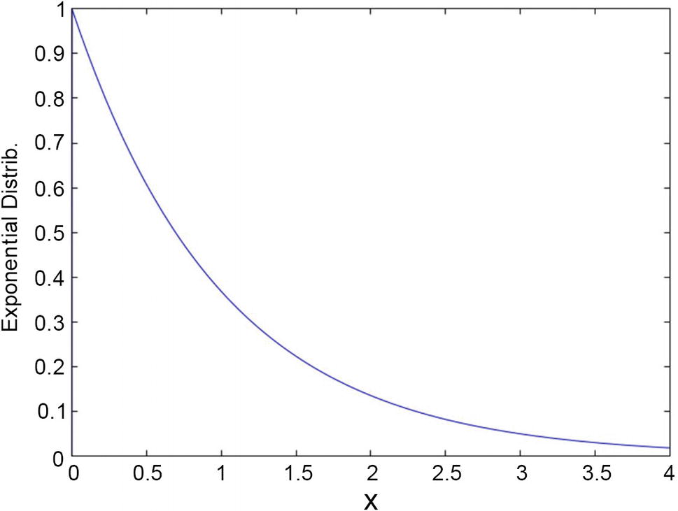
Probabilities defined by the exponential distribution, with mean 1

Probabilities defined by the Chi-squared distribution
The first step is to define a generator to use as the source of random bits. This is done by instantiating an engine (done at the file scope). The std::default_random_engine is the default generator selected by the compiler’s implementation. It should be a reasonable choice, unless you want to be very specific about the generator for your code.
The get_uniform_int function generates a random integer between 0 and max, where max is a parameter passed to the function. The function first checks if the parameter is valid and throws an exception when that is not the case. The function then uses the parameter to create an object of type uniform_int_distribution. This object receives two parameters that define the distribution: the minimum and maximum values. The resulting object is then used to generate the random number itself.
Traditional C and C++ code used to rely on the rand function to generate random integer numbers. This usage is now deprecated because the algorithm used in rand() is known to have weaknesses. In particular, the idea of using the expression (rand() % N) to generate random integer numbers in the range 0 to N-1 has been proved to be unreliable. Even though the numbers seem random enough for most applications, it fails when you try to perform more complex statistical analysis.
Find a suitable random engine and a corresponding generator according to the needs of your application.
Select a generator instantiation based on the random engine you selected previously. If you don’t have any specific requirements, the default_random_engine could be used.
Select a random distribution according to the needs of your application. A common distribution is the uniform, which produces numbers with the same probability in a given range.
Create an object of the type determined by the probability distribution. In the previous example, you used uniform_int_distribution as the object type.
The resulting object can now be called to generate pseudo-random numbers, once the generator object is passed as the single parameter for the call. This makes it possible to use generators of different types or, more commonly, generators that are used for a specific function of a thread.
Using Common Probability Distributions
This section will show a few examples of common probability distributions and how they can be used in C++. As mentioned, random numbers can be generated according to different probability functions. These families of functions are grouped according to the parameters and shape of the distribution.
One of the simplest probability distributions is the Bernoulli distribution. This is a family of probability distributions that model a yes/no scenario, an event that has only two results. The only parameter for this distribution is the probability of the yes result. The simplest example of this type of model is a coin toss, with parameter 0.5, representing a fair probability of heads or tails.
In this code, the first step is to use a generator, which in this case is std::default_random_engine allocated in the file scope, so it is available during the lifetime of the application. The coin_toss_experiment function initially checks the validity of the parameter num_experiments, which gives the number of tries in this random experiment.
The function then allocates a new object from the Bernoulli distribution, with parameter 0.5, which indicates that the yes/no event occurs with even probability for each side. The random values are then generated in the loop, where the bernoulli returns Boolean values according to the desired distribution behavior. The values are stored in a vector<bool> container.

Here, k is the number events that are observed, and λ is the parameter that determines the results of the experiment, which can be interpreted as the average number of events occurring in the given time period.
In the C++ standard library, the Poisson distribution is made available through the std:: poisson_distribution template . The parameter for this distribution is the mean, usually represented as the mathematical variable λ as in the previous equation.
The num_customers_experiment function can generate a sequence of random values based on the Poisson distribution and return a histogram of these values, that is, for each value, it returns the number of times this value was observed.
The algorithm is similar to what you have seen before with the Bernoulli distribution. The first part is used to define the random generator, and it creates an object of type std::poisson_distribution. The parameter passed represents the mean of the distribution.
The for loop in the algorithm is used to build the histogram. At each step, a number is generated according to the Poisson distribution. Then, if the resulting number is less than the parameter max, that value is incremented in the list of occurrences.
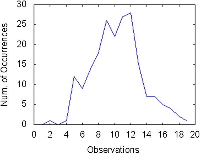
Histogram of the data returned by function num_customers_experiment
The next example shows how to generate and use random values drawn from the normal distribution. The normal distribution, also known as Gaussian distribution, is one of the most common probability distributions used to model real-world data. It is employed in data analysis, in areas ranging from drug design to sociology. The normal distribution represents the distribution of values that are naturally measured in populations. For example, the heights of people living in a particular geographical area follow the normal distribution.

In this equation, μ is the mean value of these numbers, and σ is the standard deviation, which is a measure of the variability of these random values.
The next function, test_normal, can be used to verify the correctness of this code. The idea of this function is to use the generated values so that it can create a histogram of the normal-distributed data. The first step of the algorithm is to call the get_normal_observations function and save the returned data. The next step is to get some information about the received data, such as the minimum and maximum values. This is done using the std::minmax_element function , which returns a pair of iterators pointing to the minimum and maximum values in the given range.
The algorithm creates a vector with elements corresponding to “bins,” that is, smaller ranges where each observation is recorded. The size of each such bin is stored as the variable h. The first loop then determines the number of elements in each such range so that a histogram can be calculated.
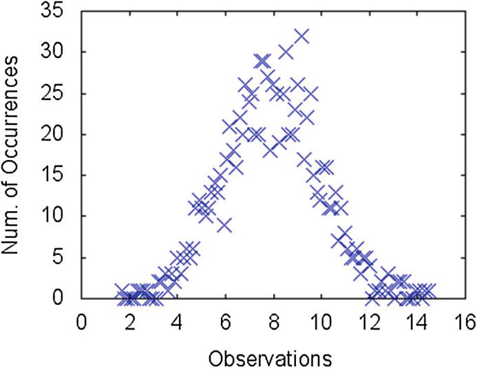
Histogram of values observed using the normal distribution with mean 8
Creating Random Walks
One of the main applications of stochastic processes in finance is the study of prices under random variations. This random process is called a random walk, since it implies that changes happen at random as time passes. A random walk model can be used to simulate market conditions and investigate the behavior of trade strategies, portfolios, and market participants in general. In this section, you see how to create a simple random walk using some of the facilities provided by C++.
A random walk can be designed with the use of a few simple rules that determine the price fluctuations. Notice the exact rules used depend on the kind of market that you need to simulate and the exact conditions that need to be replicated. In this example, I use a few computational commands that will simplify the task; the framework can be readily extended to implement more complex scenarios.
A price decrease, which occurs with probability 1/3.
A price increase, also happening with probability 1/3.
The price remains unchanged.
The amount of increase or decrease is given by a parameter called stepSize.
The number of steps, m_numSteps, determines the number of steps (time) in the random walk.
The initial price is defined by the m_stepSize member variable.
The starting price is defined by the m_startPrice member variable.

A random walk generated by the RandomWalkModel class with starting price of $30
Conclusion
In this chapter, I introduced a few examples of Monte Carlo techniques, which can be used to solve complex problems through simulation of random events. These methods are based on the use of pseudo-random values as a tool for the probabilistic analysis of events. Such models also support the simulation of complex mathematical models, including the evolution of stock prices, as well as their options and related derivative instruments.
In the preceding sections, you learned about the building blocks of Monte Carlos methods. First, you learned how to generate pseudo-random numbers using the C++ standard library. The random numbers can also be generated according to a predefined probability distribution. The C++ standard library contains some of the best-known probability distributions, which makes it easy to integrate these features into user applications.
You also saw how to implement a simple random walk model. In a random walk, values change by small increments in either negative or positive directions. The random walk model can be used to analyze several financial instruments, ranging from fixed income instruments to equities and derivatives.
The next chapter will cover additional library functions and classes that are commonly used to analyze and develop solutions for options and derivatives.