
2. Basic Current Concepts
2.1. Types of Current
Current flows take many different forms that can have useful properties and sometimes very random natures. This section describes some of the more common forms.
Sometimes it is difficult to figure out if we are graphing current or voltage. It is important to understand that there is an intimate relationship between voltage and current. Current flows because (typically) there is a difference in voltage between two points. A voltage difference between two points may create a current between those two points if a circuit is connecting them. If a circuit is present, then usually both voltage and current are associated with the circuit. The relationship between voltage and current is defined by Ohm’s Law, which is covered in a later chapter.
The wave-shape illustrations that follow are intended to represent current flows. They could just as easily represent voltage, and indeed the same discussions would apply. The purpose of this section is really to illustrate different wave shapes rather than to distinguish between voltage and current.
2.1.1. Direct Current
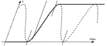
Direct current (DC) is current that flows in one direction (Figure 2-1). A battery is a good example of a power source that provides current in one direction (by convention, from its positive terminal to its negative terminal). Direct current does not mean constant current. A battery can provide current that flows only in one direction, but the amount of current that flows is determined by the circuit and can be quite variable.
2.1.2. Alternating Current
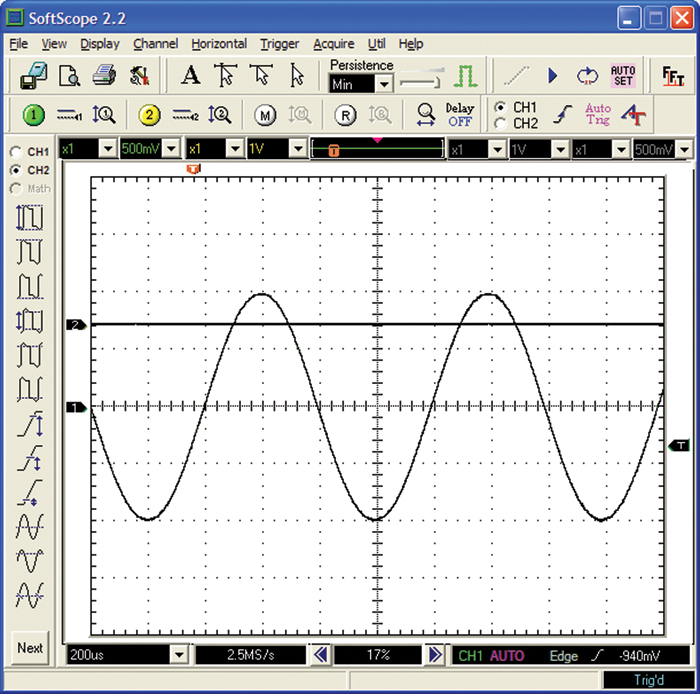
Alternating current (AC) can take many forms. We usually think of it as what comes from the outlets in our walls. In the United States, wall outlets typically provide approximately 110 volts AC at 60 Hertz (Hz). The 60 Hz (cycles per second) means that the voltage swings positive for half a cycle, then swings negative for half a cycle, as shown in Figure 2-1. Sixty of these cycles are completed each second. This means that for a brief period of time (1/120 of a second), one side of the outlet is positive relative to the other side, and then it becomes negative relative to the other side. Since conventional current flows from positive to negative, this means that current flowing from our wall sockets changes direction 120 times each second.
It is important to emphasize the word relative. The total current flow can be in only one direction, and there will still be an AC component to it. Suppose we have a current flowing down a wire that has two components: one a DC component of 1 amp and one an AC component (peak-to-peak) of 0.25 amp (250 ma). In this case, the total current flow varies between 0.75 amp and 1.25 amps. There is never a time where current completely changes direction. Nevertheless, we consider the 250-ma current flow to be an AC current (250 ma peak-to-peak) component superimposed on a (1-amp) DC current bias.
Figure 2-1 illustrates a sinusoidal current waveform. AC does not necessarily imply sinusoidal. Any current waveform that changes magnitude has an AC component. It may be a regular, repetitive waveform, as shown, or a completely random waveform, as we’ll see later.
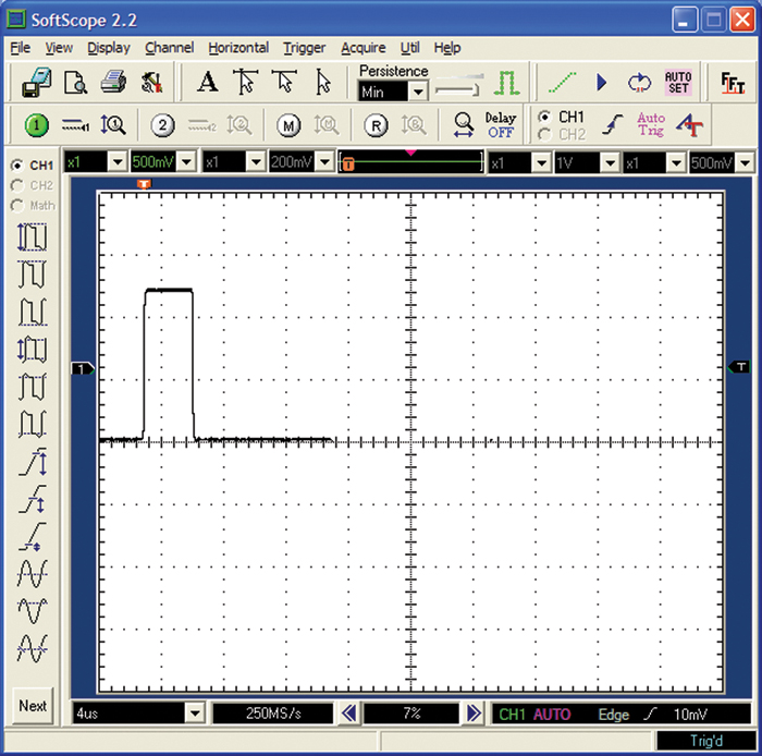
2.1.3. Step Functions
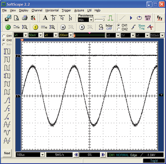
When a current (or voltage) changes quickly from one level to another, we refer to the change as a step-function change. A control signal that is either “on” or “off” (“high” or “low”) typically goes through a step-function change. Figure 2-2 shows a step-function change from a low to a high level.
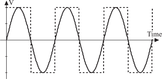
2.1.4. Square Waves
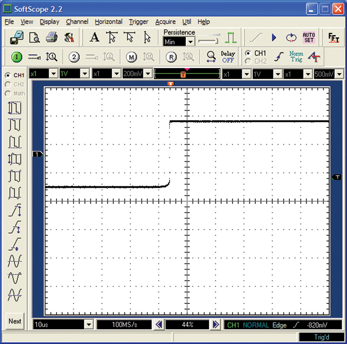
A square wave is a special case of an alternating current where there is a repetitive step-function change in current from one level to another. In many digital circuits we have a clock signal. The “ideal” clock signal wave shape is square, as shown in Figure 2-3. We sometimes talk about the magnitude of this signal in terms of its logical components—that is, whether it is on and off, or logical one or logical zero—instead of its voltage or current magnitude. Typically a square wave ranges from zero to a positive value, or between a plus value and a negative value. In one sense, a square wave is just a regularly repetitive step change.
2.1.5. Pulses
One form of a current pulse is shown in Figure 2-4. This pulse looks like a square wave with some missing parts, or what we call a low duty cycle. A pulse might represent that a particular event has happened—for example, a key on a keyboard has been pressed. A series of pulses may represent coded information, as in a bit stream or a data stream.
2.1.6. Transients
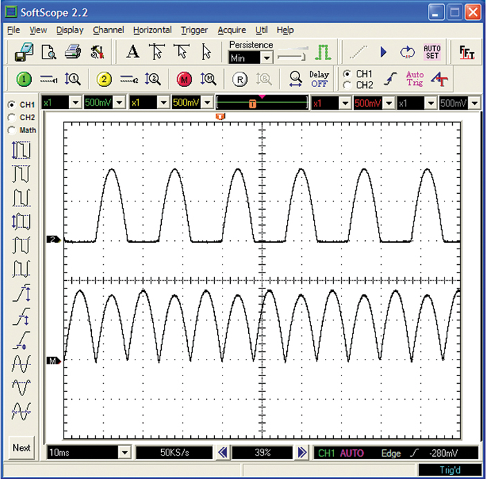
The word transient usually implies a short-term reaction to some form of impulse. A transient current usually is the result of some other stimulus. For example, the transient current shown in Figure 2-5 is the current flowing into a capacitor caused by a step-function change in voltage.
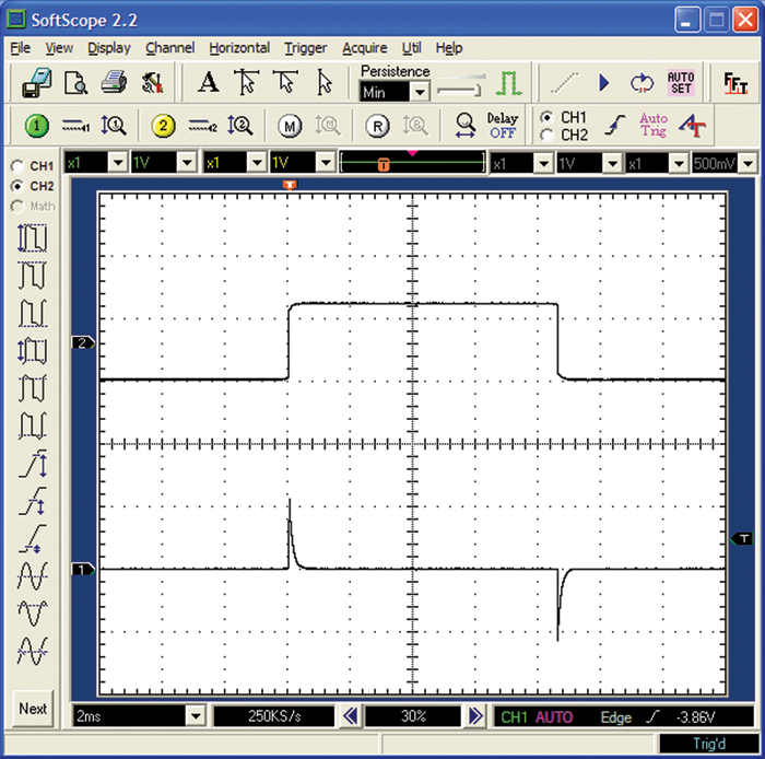
Figure 2-5 Transient current flow into a capacitor (lower curve) caused by step-function changes in voltage across the capacitor (upper curve).
2.1.7. Complex
A sine or cosine waveform is a standard waveform that occurs in nature. These waveforms belong to a more general class of waveforms called trigonometric. Many objects in nature follow trigonometric paths: a bouncing ball, ocean tides, and the movement of planets around the sun. Formulas have been derived through the centuries to analyze trigonometric behavior.
Other waveforms are not natural in the sense that they do not occur naturally. A square wave clock pulse (Figure 2-3) is a particularly relevant example. In electronics, single-frequency trigonometric waveforms (sine and cosine, for example) can be analyzed with available formulas and have already been derived for handling natural phenomena. A square wave, however, does not lend itself to easy analysis. How, then, can we analyze circuits with more complex waveforms?
The answer is that we can first convert a complex waveform into a series of trigonometric waveforms and then analyze the circuit for each of the individual single-frequency waveforms in the series; finally, we add up these analyses. This sounds very tedious and complex, and indeed it can be. Engineers do, however, have higher-order mathematical tools to help them.
The conversion of a complex waveform to a trigonometric series is based on something called Fourier’s Theorem, which is as follows:
Every signal or curve, no matter what its nature may be, or in what way it was originally obtained, can be exactly reproduced by superposing a sufficient number of individual sine (and/or cosine) waveforms of different frequencies (harmonics) and different phase shifts.
This means that any waveform (in theory it must be a repetitive waveform, but in practice we often wink at that requirement) can be reproduced by superimposing a sufficient number of sinusoidal waveforms at higher-frequency harmonics. So we take a look at our input waveform of interest (perhaps a video signal, perhaps a complex digital signal formed by a series of square waves and pulses) and reproduce it with a series of sinusoidal waveforms (which Fourier’s Theorem says we can do). Then we analyze the performance characteristics of our circuit for each one of the individual sinusoidal waveforms. Finally, we add up (superimpose) all of these results to get the combined result of the circuit to our input waveform.
Let’s look at some examples. Although a square wave is not a natural waveform that exists in nature, we can use a Fourier transform to represent it as an infinite series of cosine or sine waves. One form of a square wave series is as follows:
Each component (term) in the series shown in Equation 2.1 represents a harmonic of the fundamental frequency, θ. As it happens, a square wave, when represented by this cosine series, only contains odd harmonics. Figure 2-6 illustrates what happens as we use progressively more terms (harmonics) to represent the function. Each additional harmonic makes the resulting waveform look a little more like a square wave.
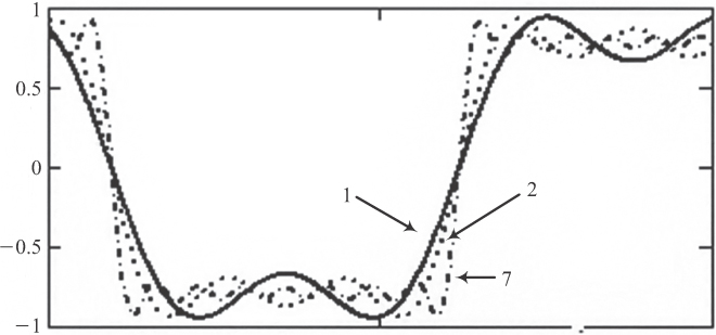
Figure 2-6 As we add more harmonics to the series, a better approximation to a square wave results. These series are for one harmonic (1), two harmonics (2), and seven harmonics (7).
Figure 2-7 shows an example of this same series carried out to 101 harmonics (2 × 50 + 1). The example was created using Mathcad, a readily available software package available from Mathsoft, Inc. If you have Mathcad software, you can replicate this example on your own.
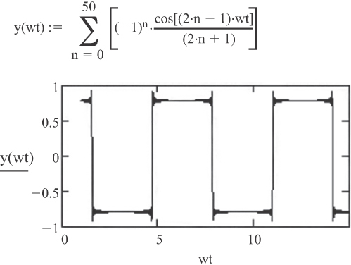
A simulation program called Square.exe is available on the UltraCAD Web site.1 It allows you to explore this cosine series in some detail and see how various assumptions affect the nature of the waveform.
1. See www.ultracad.com/simulations.htm.
Figure 2-8 illustrates various series for forming other standard waveforms. What is instructive here is that any waveform can be “decomposed” into a series of sinusoidal harmonic terms that can then (at least conceptually) be individually analyzed and then added together to determine the response of a circuit. Again, conceptually this is straightforward, but in practice, it can be quite difficult and involves very complex math and calculus.
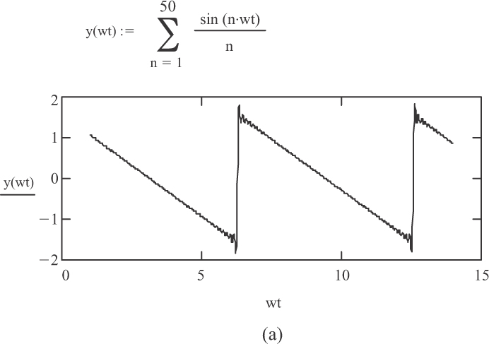
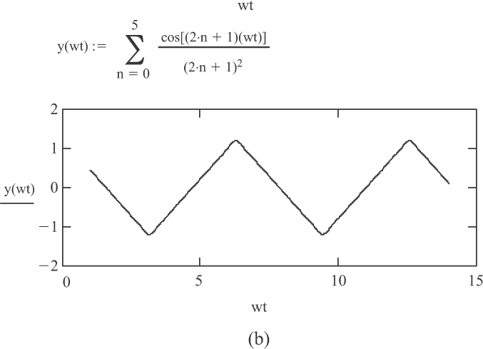
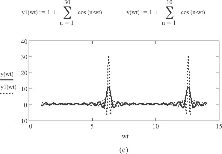
Figure 2-8 Fourier series for three common complex waveforms: (a) sawtooth, (b) triangular, and (c) pulse.
2.1.8. Random Current Flows
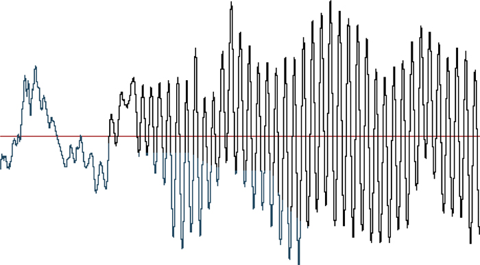
Finally, some types of current flow can best be described as random, or at least nonperiodic or nonrepetitive. They probably are not random in the strictest sense, because if the current represents a signal of some sort, there is coherent information contained within the signal. But dealing with that information typically requires processing. Prior to processing the signal, the current can appear to be pretty random.
Figure 2-9 shows an example of this. This illustrates a portion of an audio signal. Many frequency components are contained within this waveform, and each has its own amplitude and phase. Engineers have algorithms available to them for analyzing complex waveforms such as these, but the algorithms themselves are very complex and usually require considerable processing power.
2.2. Propagation Speeds
Electrical signals traveling along a conductor in the air travel at the speed of light: 186,280 miles per second (which, if you do the math, comes to 11.8 inches per nanosecond (in/ns)). That speed is equivalent to 7.5 trips around Earth’s equator in one second. Yet, we have to worry about how fast these signals travel along traces on our boards! That is pretty amazing when you think about it.
Consider this experiment: Say you suspended a copper wire across a lake and measured how long it took a signal to travel from one end of the wire to the other end. Now say you lower the wire into the water and measure the signal propagation time again. What do you think would happen to the propagation time?
When a current flows along a conductor, it generates an electromagnetic field around the conductor. This electromagnetic field has two components: an electrical field and a magnetic field (see Sections 1.4 and 1.5 in Chapter 1). The electrical field originates with the charged electrons. It radiates radially out from the conductor with a strength that decreases with the square of the distance from the conductor. The magnetic field originates from the motion of the electrons along the conductor. There is no magnetic field if there is no motion (current). The strength of the field changes with the magnitude of the current. The magnetic field radiates around the conductor with a polarity that depends on the direction of the current and with a strength that is inversely related to the square of the distance from the conductor.
The electromagnetic field and the current must move together. The current can’t move out in front of the fields, and the magnetic field can’t move out in front of the electric field. It turns out the issue is not how fast the current (electrons) can flow through the conductor but how fast the electromagnetic field can flow through the medium it is flowing through—the medium around the wire.
All materials have a characteristic called the relative dielectric coefficient (∊r), which is a measure of the material’s ability to store charge. It is called relative because it is referenced to the dielectric coefficient of air (really that of a vacuum, but the difference between air and a vacuum is so small that only astronomers really care). Its relevance here is that the speed with which an electromagnetic field can travel through a material is equal to the speed of light divided by the square root of the relative dielectric coefficient of the material. Therefore, the propagation speed (in in/ns) of a signal is given by the formula in Equation 2.2.
So let’s go back to our experiment with the wire dropped into the lake. Again, the issue is not how fast the electrons can travel through the copper wire but how fast the electromagnetic field can travel through the water. The relative dielectric coefficient of water is approximately 80 (depending on its purity), and the square root of 80 is approximately 9, so the signal will slow down when the wire is lowered into the water by about a factor of 9.
2.2.1. Propagation Times
It is easy to confuse propagation speed and propagation time. Propagation speed means velocity, and the units are distance per unit time. Propagation time is, well, time. A related measure, wavelength (the distance a signal travels in one complete cycle), is discussed later in this chapter. We express propagation time either in units of time (e.g., nanoseconds) or as units of time per unit length (e.g., nanoseconds/inch). Propagation time (expressed as time per unit length) is the inverse of propagation speed, as follows:
Propagation Time (per unit length) = 1/Propagation Speed, or
Propagation Time = Length/Propagation Speed
For example, if an electrical signal in a copper wire in air travels at the speed of 11.8 in/ns, then it propagates down the wire at 1/11.8 or 0.085 ns/in.
2.2.2. Trace Configurations and Signal Propagation
Figure 2-10 shows some trace configurations that designers usually work with when designing high-speed boards. Most boards in situations where signal integrity is an issue have internal planes. From a signal propagation standpoint, traces that are located between two reference planes are considered to be in a Stripline environment, regardless of whether the actual environment is a simple, centered, dual, offset, or asymmetric Stripline configuration. A trace with a reference plane on only one side is considered to be in a Microstrip environment.
Figure 2-10 Common trace configurations on PCBs: (a) Microstrip, (b) embedded Microstrip, (c) Stripline, (d) dual Stripline, and (e) asymmetric Stripline.
A Microstrip trace might simply be an external trace with air above it, and board material between it and an underlying plane. An embedded Microstrip trace also has board material above the trace. This would particularly be the case if two external trace layers were above the plane. In that case, at least the traces on layer 2 would be embedded Microstrip traces. A coated Microstrip trace would be one with board material between it and the reference plane and with an additional material coating above the trace. The additional coat could be a variety of materials, including solder mask, conformal coating material protection, and so on.
We generally consider the material surrounding a trace in a Stripline environment to be homogeneous (uniform). In fact, we usually specify it to be this way. Therefore, the propagation speed of a signal in a Stripline environment is dependably expected to be as described in Equation 2.3.
Actual experience generally only varies from this calculation if the ∊r is not as expected or if the material is quite nonuniform. Since the relative dielectric material of FR4 is approximately 4, and since the square root of 4 is 2, the propagation speed of a signal in a Stripline environment is often considered to be 11.8/2 ≈ 6 in/ns, a relationship we are all familiar with. If we want to be more precise in our calculations, then we have to know the relative dielectric coefficient of the material we are using more precisely and plug that value into Equation 2.3.
The Microstrip environment is more problematic. The material surrounding the trace is not uniform. In the simplest case it is air above the trace and dielectric below the trace. In more complex cases the dividing line between the dielectric and the air might not be precisely uniform, and there may be more than one type of material involved.
Therefore, if you want to estimate the signal propagation speed in Microstrip, you need to estimate the effective dielectric coefficient of the material surrounding the trace. A generally accepted rule of thumb for estimating the effective dielectric coefficient is provided in Equation 2.4.
There are a couple of problems with this estimate. The most significant one is that it is a constant. People have discovered that propagation time in Microstrip is a variable and, all other things being equal, is a function of trace width and height above the plane.
As trace widths get wider, propagation speed slows down! This is because as traces widen, a larger percentage of the field lines between the trace and the plane is contained within the dielectric. In the limit, with infinite trace width, virtually all of the electromagnetic field is contained within the dielectric. In this case, the Microstrip trace behaves very much like a Stripline trace.
Microstrip propagation speed also slows down as the trace gets closer to the plane for the same reason. A greater percentage of the field lines is contained within the dielectric than in the air. Brooks has shown that a much better estimate of propagation time in Microstrip can be obtained by expressing it as a ratio times the propagation time for a signal in a Stripline environment surrounded with the same dielectric material. He created a formula for estimating this ratio.2 The propagation time for a Microstrip trace will never be longer than for a trace in a Stripline environment surrounded by the same material. It may be shorter, depending on how the electromagnetic field splits between the air above the trace and the dielectric under the trace. His estimate for propagation time (in ns/in) is as follows:
2. See “Propagation Speed in Microstrip: Slower Than We Think” at www.pcbdesign007.com/pages/columns.cgi?artcatid=0&clmid=55&artid=76489&pg=1.
Propagation time(Microstrip) = Br × Propagation Time(Stripline)
or
where:
Br = 0.8566 + (0.0294)Ln(W) – (0.00239)H – (0.0101) ∊r ≤ 1.0
W = trace width (mils)
H = distance between the trace and the plane (mils)
∊r = relative dielectric material between the trace and the underlying plane
Ln represents the natural logarithm, base e
The fraction, Br, can never be greater than 1.0. A Microstrip trace can never be slower (i.e., propagation time longer) than a Stripline trace (surrounded by the same material). The formula was derived for simple Microstrip traces with air above the trace and dielectric material underneath. Embedded and coated Microstrip traces would have slightly higher fractions (and slightly slower propagation times) than estimated here, subject to an upper limit for the fraction, Br, of 1.0.
2.3. Circuit Timing Issues
“Timing is everything,” as the saying goes. In complex circuits we have signals on buses running everywhere. There are certain moments in time when those signals must align exactly right. Here are a few examples of those times.
1. The three colors of a video display (red, green, and blue) must arrive at a receiver at the same time or the video picture will be distorted.
2. The two traces of a differential pair must be the same length so that the two opposite signals arrive at the receiver at the same time or common mode noise may be generated.
3. The data lines must be present and stable at their respective gates when the clock pulse triggers or there will be data errors.
Figure 2-11a shows what might happen if there is a timing problem. Three signal lines are shown, with the top line slightly misaligned from the others. A clock pulse samples the data state. The data signals don’t line up quite right, but the clock signal still samples the data signals when they are all high or all low. In Figure 2-11b, however, the middle signal is so badly misaligned that it transitions during the time the clock is sampling the data lines. In Figure 2-11b there will be data logic errors.
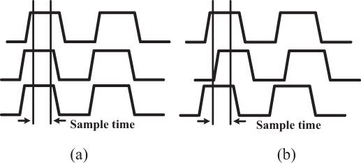
Figure 2-11 Circuits can tolerate slight differences in timing (a), but if the differences in timing are too great, sampling errors will occur (b).
Signals get misaligned for several reasons, one of which involves the devices themselves. There is a throughput time for a signal to travel through a device and tolerances on the output timing of devices. The circuits have different numbers of devices through which the signals propagate. There are propagation delays on the traces, but at certain well-defined points and times in a circuit and system, certain signals must align properly. The circuit design engineer is responsible for creating the specification for this, but the board designer may be responsible for making it happen.
Board designers control signal timing with trace length. Multiplying the propagation time (in units of ns/in) of a trace by its length gives the propagation time of the signal down the trace. If we need the trace to be a specific increment of time, then we adjust its length to make it so. This process is often called tuning the trace.
Adjusting timing this way requires two things: a precise knowledge of the propagation speed of the signal along the trace we are interested in and the ability to adjust the trace length. We determine the propagation speed from the preceding discussion. Inherent in the determination is the knowledge of the relative dielectric coefficient (∊r) of the material surrounding the trace. We cannot make the trace shorter than the distance between its connection points, but we can make it longer. The normal way to adjust trace length is to “snake” it.
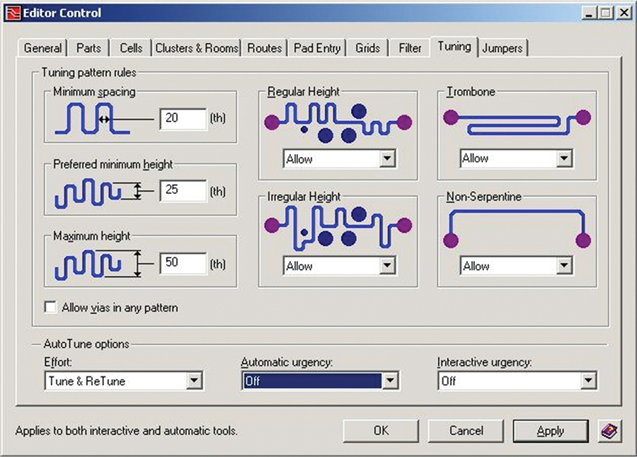
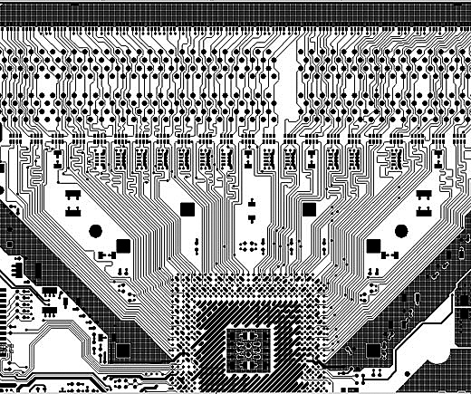
Many of the higher-end PCB design programs will automatically adjust trace length once you give it the appropriate parameters. Figure 2-12 shows the tuning editor from one of them. Note the variety of patterns the designer can specify. Figure 2-13 shows a portion of a board that required a considerable amount of tuning.
Some engineers worry about EMI radiation that might be caused by tuning patterns. In our experience we have seen no EMI issues from any type of tuning pattern as long as (a) every trace is referenced to a signal plane and (b) the tuning is confined to Stripline signal layers. Lots of traces are successfully tuned on Microstrip layers (look at almost any computer motherboard), and we do it all the time. But if you or your engineers have significant concerns about tuning causing EMI problems, confining tuning to inner layers will almost always eliminate any possibility of radiation.
Some articles suggest that crosstalk between segments of tuning loops can interact with the signal propagation speed and distort timing calculations. This is probably a concern only with narrowly spaced serpentine traces at the highest clock speeds and is beyond the scope of this book.3 People debate whether via length should be taken into consideration while calculating propagation time, but there does not seem to be a definitive conclusion in the industry one way or the other about this.
3. See, for example, Brooks’s article “Adjusting Signal Timing, Part 2” at www.ultracad.com/mentor/mentor%20signal%20timing2.pdf.
2.4. Measures of Current
At first glance, the idea of a measure of current seems fairly basic. Saying that a 1MHz AC current is 1 amp would seem to be pretty descriptive. But it can be much more complex than this. This section looks at a variety of different measures that can apply to current, and the meanings can be quite different, depending on what measure is used.
2.4.1. Frequency
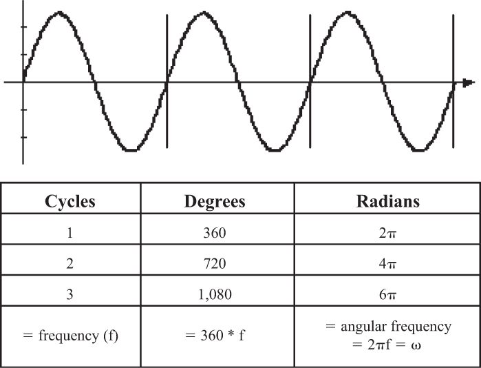
We can measure, or refer to, frequency in three ways. The most common one is in cycles per second, or Hertz, often designated by the symbol “f.” Thus, the waveform shown in Figure 2-14 has a frequency of 3 Hertz, or f = 3. This is a very common measure of frequency. We can also refer to the number of degrees the waveform goes through in one second. A sine wave completes 360 degrees in one cycle, so in three cycles it completes 360 × 3 or 1,080 degrees. Thus, the waveform in Figure 2-14 could be said to have a frequency of 360 × f or 1,080 degrees/second. In general we could describe any frequency as 360 × f degrees/second. However, we almost never use this measure of frequency.
But there is a related measure of angular frequency we do use. We start by dividing the circumference of a circle into radians. A radian is the angle formed by a length along the circumference of a circle equal to the radius of the circle (Figure 2-15). Take a length equal to one radius and lay it along the circumference. Look at the angle formed by the beginning and the end of this length (arc). That angle (α) is defined as a radian.
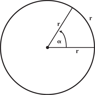
The circumference of a circle is 2πr, where r is the radius. So if we ask how many radians there are in a circle (360 degrees), the answer is
Circumference/radian = 2πr/r = 2π
So 2π radians make up a complete circle (360 degrees).
Since there are 2π radians in 360 degrees, there are 2πf radians completed by a sine wave in one second. This measure of frequency is one we do use in electronics, and it is given a special symbol, ω, as shown in Equation 2.6.
This measure of frequency is called the angular frequency or angular velocity, and it shows up in a great many formulas used in electronics. It measures the number of radians a sine wave goes through (completes) in one second.
If a typical AC waveform (voltage or current) is of a single frequency and is trigonometric in nature, then it can be represented by the term sin(x), where x is a measure of frequency. We typically represent such a waveform by the expression sin(2πf t) or sin(ωt), where 2πf or ω represents the number of cycles in one second and t represents the time variable (in seconds)
2.4.2. Harmonics
Let’s say we have a signal with a certain frequency and we can describe that waveform by the relationship
where ω is a measure of frequency and t is a measure of time. Then a waveform whose shape is given by the formula V = sin(2ωt) has twice the frequency of the first waveform, and another waveform V = sin(3ωt) would have three times the frequency.
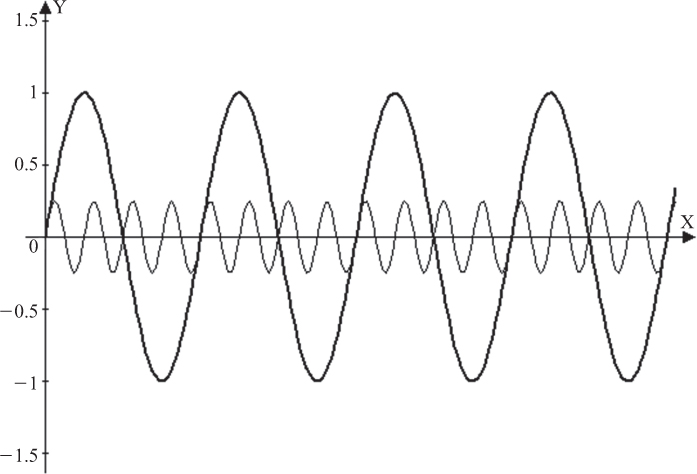
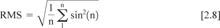
We can generalize this by saying that a waveform with shape V = sin(nωt) has a frequency n times higher than a waveform whose shape is V = sin(ωt). If the waveforms are related to each other (perhaps the sin(nωt) waveform was somehow generated by the sin(ωt) waveform, or perhaps they were both generated by the same source), then such shapes (waveforms) are called harmonics. Harmonics are simply multiples of the base, or fundamental, frequency. In this case the sin(nωt) signal is called the nth harmonic of the fundamental sin(ωt) signal. Figure 2-16 shows a signal and its fourth harmonic (reduced in amplitude). Harmonics are very important in electronics and, in particular, signal integrity.
2.4.3. Duty Cycles
Whenever we have a repetitive signal, such as the AC waveform in Figure 2-1, the square wave in Figure 2-3, or the pulse in Figure 2-4, the signal spends part of a cycle in the positive, “high” or “on” state and part of the cycle in the negative, “low” or “off” state. Duty cycle refers to what percentage of the time the signal is in the high state. For example, a typical square wave is high 50% of the time and low 50% of the time. We say that it has a 50% duty cycle. A signal that is high only 25% of the time is said to have a 25% duty cycle. Figure 2-17 shows examples of both.
Usually a signal only dissipates power when it is in the high state (this may not always be true, depending on the circuit). Duty cycle then becomes a way of evaluating the power dissipation of two different signals. One signal with a 60% duty cycle, for example, will dissipate twice the average power of a signal with a 30% duty cycle.
2.4.4. Rise Times
Frequency is the measure of how many times the current cycles through a change in direction in one unit of time (usually one second). Thus, the smaller curve in Figure 2-16 illustrates a higher frequency than does the larger waveform. If the horizontal axis in the figure represents one second, then the larger waveform has a frequency of four cycles per second (or 4 Hertz) and the smaller waveform has a frequency of 16 Hertz. We now commonly see waveforms on our circuit boards with frequencies in the range of hundreds of millions cycles each second (hundreds of MHz), and sometimes much higher. That means the AC waveform, or the current, is cycling back and forth, or changing direction, hundreds of millions of times each second!
It is a common misconception that frequency is the most important issue in high-speed designs. Rise time is the real culprit. Figure 2-18 shows two waveforms: a sine wave and a square wave. Each of these waveforms has the same frequency, but they have significantly different rise times.
Rise time is normally defined as the length of time required for the waveform to rise from the 10% point on the waveform to the 90% point (Figure 2-19). Occasionally you will see rise time defined between the 20% and 80% points. Fall time is defined exactly the same way: the time for the waveform to fall from the 90% point to the 10% point. If you superimposed a sine wave alongside the rising edge of a signal, as shown in Figure 2-19, it can be shown that the 10% to 90% portion of a sinusoidal waveform is just about one-third the time for a complete cycle, or period, τ, of the waveform. You might say that for a sine wave the relationship is Tr = 1/(3f), where Tr = the rise time and f = the frequency in Hz.
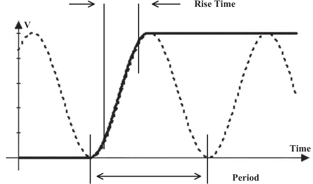
Figure 2-19 The rise time of a pulse is approximately 30% of the period of the underlying sine wave.
Technical Note
Some books define this relationship as Tr = 1/(πf).
You might ask why we refer to the 10% to 90% range of amplitude for rise time and not the 0% to 100%. Or why do some use the 20% to 80% measure for rise time? The answer may be somewhat less than satisfying, but it goes like this: Almost all switching devices follow a switching pattern similar to that shown by the rising line in Figure 2-19, but they may differ significantly in the very first or last portions of their switching pattern. For example, one type of device may reach 100% very quickly, but another device may roll off as it approaches the 100% level and actually may not reach 100% for several moments (we sometimes say it may approach 100% asymptotically). Switching devices might have quite different switching patterns in the very beginning or ending stages of their switching range, but usually all have quite similar patterns during their main transition. Therefore, we use the 10% to 90% points of the switching range for the rise time measure in order to compare “apples to apples.” Sometimes others may use the 20% to 80% range because the beginning and ending parts of the switching range are a little “broader” than other devices or because they are engaging in “specsmanship” (the 20% to 80% range is shorter and therefore seems faster).
Suppose we have a voltage or current requirement in a circuit that changes rapidly. For example, suppose we have a current requirement that goes from 0 mA to 10 mA within 1 ns. We can express this requirement as a “change in current divided by a change in time,” or Δi/Δt (where Δ means change). If we consider the relationship Δi/Δt and think of Δt as an extremely short period of time, then we would mathematically express the relationship as di/dt (pronounced dee-eye-dee-tee). The term di/dt is a calculus expression that means “the change in current divided by the change in time as the change in time becomes vanishingly small”—that is, as Δt becomes really small! In extremely fast circuits, the term dt equates to the rise (or fall) time of the signal. It is this di/dt term that causes the signal integrity problems.
We in the industry often simply use the term rise time generically to describe a circuit requirement. The reader should understand that fall time is equally important. What is really important is the faster of the two. So when you read “rise time” think “rise or fall time, whichever is faster.”
2.4.5. Periods
The time required for a single cycle is 1/f, where f is the frequency. The time for a single cycle is called the period (τ). So a sine wave with a frequency of 1MHz (1 million cycles in a second) has a period of 1 millionth of a second, or 1 μs, or 1,000 ns. Therefore, the rise time of a 1MHz sine wave is about one-third of that, or about 333 ns.
2.4.6. Phase Shifts
When we use the term phase in electronics, we are usually referring to an AC trigonometric (sine or cosine) waveform. When we talk about phase shift, we are referring to a difference in time between two similar waveforms. For example, we talk about a phase shift between voltage and current at a particular (sinusoidal) frequency at a particular point in a circuit at any given point in time. It is important to note that phase shift usually is not related to signal timing issues. If a device has two input pins, we usually don’t refer to the difference in signal timing between the pins as a phase shift. Instead, we might refer to that as a signal offset.
If two AC waveforms peak at the same point in time, we say they are exactly the same phase, or are in phase. Figure 2-20a shows two waveforms that are in phase. If they peak at different points in time, they are no longer in phase. One waveform will peak before the other one. We say that the waveform that peaks earlier leads the other waveform or that the second waveform lags the first waveform. Figure 2-20b shows two waveforms that are not in phase.
Figure 2-20 The top and bottom curves in (a) are in phase. The top curve leads the bottom curve in (b) by about 90 degrees.
There are a few absolute truths we must remember. Voltage and current are always exactly in phase in a resistor. Current leads voltage by 90 degrees in the case of capacitors. Current lags voltage by 90 degrees through an inductor. It is important to understand that these three statements are always true (as long as we are talking about ideal capacitors and inductors, those with no internal resistance). There are no exceptions. Therefore, if we have both inductors and capacitors in a circuit, it is possible to have a 180-degree phase shift between two signals (+90 for the inductor and –90 for the capacitor can sum to a difference of 180). Under exactly the right circumstances, two signals that are 180 degrees different in phase can exactly cancel, causing some unusual and special effects. We will learn much more about all this in Chapters 5, 6, and 7.
If we have resistors and capacitors (and/or inductors) in a circuit, we can then have phase shifts of any degree. Figure 2-21 shows a case where the top waveform leads the other by about 45 degrees.
2.4.7. Amplitude: Peak-to-Peak
Many people get confused by the different measures of amplitude that are used in electronics. With a DC waveform, the amplitude is pretty straightforward. It is what it is! But there are several different measures that are used with AC waveforms. In the example in Figure 2-22, the peak-to-peak amplitude of the AC signal is about 4 major divisions on the graph.
2.4.8. Amplitude: Peak
The peak amplitude of an AC waveform is one-half the peak-to-peak amplitude. It is the amplitude between the horizontal “middle” (or average) of the waveform and its peak value. In Figure 2-22 the peak amplitude is 2 divisions.
2.4.9. Amplitude: Average
The average amplitude of a symmetrical AC waveform is always zero! That is because the waveform has an equal area above and below the horizontal midpoint of the waveform. Therefore, the average value of an AC waveform is a meaningless measure.
It is possible for an AC waveform to be superimposed on a DC waveform. For example, suppose the waveform in Figure 2-22 was superimposed on a DC waveform whose value was 10 divisions (on the graphical window). One could argue that the average value of the waveform was then 10 divisions. While this is not entirely incorrect, it is a poor way to describe the measure. It is more correct to say that the average value of the AC component of the waveform is zero superimposed on a 10 division DC component.
2.4.10. Amplitude: RMS
The standard measure we use for the amplitude of an AC waveform is called the RMS value. RMS stands for Root-Mean-Square. Conceptually, we find the RMS value by breaking up the waveform into a large number of small sections and then (a) squaring the amplitude of the waveform for each section, (b) calculating the mean value of all of these squared values, and (c) taking the square root of this mean value. Mathematically we represent the RMS value of a waveform with Equation 2.8.
If the peak value of the waveform in Figure 2-22 is 2 divisions, it works out that the RMS value of that waveform is 1.414 divisions. In general, the RMS value of a sine or cosine waveform is 0.707 times the peak value. That means that the 117-volt AC waveform in our homes, for example, has a peak value of 117/0.707 = 165.5 volts and a peak-to-peak value of 331 volts.
The true RMS value of any waveform actually relates to power. Suppose we applied the sine wave voltage waveform in Figure 2-22 across a resistor. The RMS value is the equivalent DC voltage that would generate the same power (i.e., heat) in the resistor. Thus, a DC voltage of 1.414 divisions across a resistor will heat the resistor exactly the same amount that a 2-division (peak) sine wave would.
But this value, 0.707, is only the true RMS value for a sine or cosine wave. What if the waveform were a different shape? Or what if the waveform were random? The audio waveform shown in Figure 2-9 seems pretty random when you look closely at it. How could we then measure its RMS value? We discuss this question in Section 2.5.
2.4.11. Amplitude: Rectified
Almost all power supplies start with an AC power source (often our wall outlets), use a transformer to change the voltage level, and then pass the current through a diode circuit to convert the AC current to a form of DC current. The process is called rectification, and a diode historically was referred to as a rectifier. A single diode produces a half-wave rectified waveform (top waveform in Figure 2-23), and a diode bridge circuit produces a full-wave rectified waveform (bottom). These diode circuits are covered in Chapter 13.
While the average amplitude of a sine wave is zero, the average amplitude of a rectified sine wave is not. The average value of a half-wave rectified sine wave is 0.318 times its peak value. For a full-wave rectified waveform, the average is 0.637 times the peak value. The RMS value for a full-wave rectified sine wave is the same as for an unrectified sine wave: 0.707 times the peak value. This is because the sine wave and the full-wave rectified sine wave will deliver the same power to a resistive load. The RMS value for a half-wave rectified sine wave is one-half that, or 0.369 times the peak value.
2.4.12. Amplitude: dB
The concept of a decibel (dB) is sometimes difficult for students to grasp. The primary unit, bel, is named after Alexander Graham Bell. The unit we commonly work with is the decibel (deci = 1/10). There are 10 decibels in one bel.
Remembering three things about decibels will make the whole topic easier to understand.
1. It is a ratio measurement, not an absolute measurement.
2. It relates directly to power, not individual voltages or currents.
3. It is a logarithmic measure (common log, or base 10).
A bel is defined as the log of the ratio between two levels of power, P1 and P2.
Since the number of decibels is 10 times the number of bels (since one dB equals one-tenth bel), then
As an example, suppose we have an amplifier with a 12-dB gain. If it has a 0.5-watt signal in, what is the power of the signal out of the amplifier?
If:
12 = 10log(P2/0.5)
1.2 = log(2*P2)
2*P2 = 15.85
P2 = 7.9 watts
We will see in Chapter 4 that power is a function of the square of the voltage or current. Therefore, we could express Equation 2.10 as a ratio of squared voltages.
dB = 10log(V22/V12)
or
This expression is valid if the impedance related to V1 is equal to the impedance related to V2. If you are familiar with logarithmic operations, this becomes
Equations 2.10 and 2.12 are very common in electronics. You may sometimes see the meters of electronic measurement devices scaled in dB. It is important to recognize that if so, there is an implied reference power, voltage, or current level for the measurement. The reference level should be indicated on the meter face and will certainly be specified in the accompanying documentation.
2.4.13. Time Constants
A related measure to amplitude is called a time constant. It relates to the length of time it takes a waveform to change a certain percentage of the total change that will take place. For example, the lower curve in Figure 2-24 shows a very common waveform seen in electronics. It often relates to the charging or discharging of a capacitor or an inductor. This type of curve follows a very well-defined formula.
Figure 2-24 Certain types of transient responses (lower curve) follow very well-defined time constants.
Consider the length of time it takes the lower curve to change from its largest (positive or negative) value to the baseline. It will change 63% of that value in a unit of time called one time constant, 87% of the value in two time constants, and 95% of the value in three time constants. If we knew how to calculate the time constant, we could build timing circuits that know this relationship. Well, it turns out we do know how to calculate time constants, and we cover this topic in much more detail in Chapter 10.
2.5. Measurement Techniques
Current measurement for more than a century has been based on the principle of the galvanometer. The galvanometer works on the principle that a current in a coil exerts a force on a magnetized needle. This was first discovered in 1820 by Danish scientist Hans Christian Oersted. In that same year, French physicist André Ampère took Oersted’s discovery and applied it to the measurement of current, thereby inventing the galvanometer. Ampère suggested that the device be named after Luigi Galvani, an Italian pioneer in the study of electricity.
In 1880, Jacques-Arsene d’Arsonval (1851–1940) made a dramatic improvement in the design of the classic galvanometer, and analog meter movements have been described as d’Arsonval movements ever since.
2.5.1. Analog Meters
Figure 2-25 shows a d’Arsonval movement. It consists of a coil through which the current to be measured passes. A needle (pointer) is attached to the coil. The coil is pivoted in the center and is placed between two magnets, as shown. The current passing through the coil generates a magnetic field whose north pole points in the direction of the pointer. The induced magnetic field causes the pointer to rotate clockwise away from the magnet’s north pole and toward the magnet’s south pole. A spring provides tension, pulling against this rotation. Thus, the degree of rotation is directly proportional to the strength of the magnetic field, which is directly proportional to the magnitude of the current.
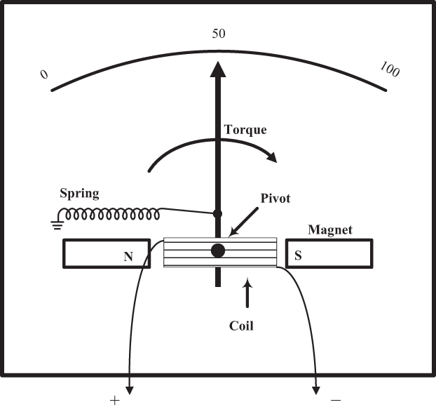
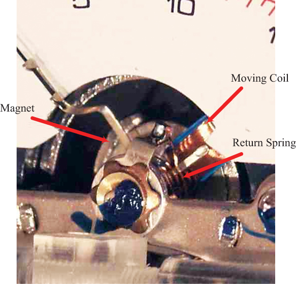
Figure 2-26 is a close-up photograph of an actual modern-day analog meter showing the components of the d’Arsonval movement.
The simplest form of current measurement is to place an analog meter directly in the current path. For example, in Figure 2-27, if you wanted to measure the current flowing around the loop (a), you would break the loop and insert a simple analog meter in the current path (b).
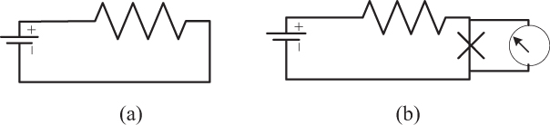
Three aspects of this approach can be troublesome. First, the current path must be broken at the point where the measurement will take place. This can be inconvenient in some instances, virtually impossible in other cases, and perhaps very unsafe in still other cases. Second, meters have limited ranges. Although you could theoretically manufacture a meter with any measurement range, meters typically move from zero reading to full-scale reading over a range from 50 μa (0.00005 amp) to 400 μa (0.0004 amp). Third, inserting a meter directly into the circuit could influence the circuit itself. The meter movement has some resistance, perhaps only fractions of an ohm to a few ohms, but this can be enough to dramatically change the performance of some circuits.
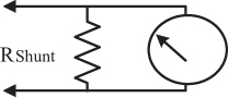
Figure 2-28 shows one way of working around the range question. A shunt resistor is placed in parallel with the meter movement, forming a current divider. If the shunt is very low resistance (0.025 ohms is not an unreasonable value), then most of the current will pass through the shunt, probably having little effect on the rest of the circuit. Still, enough current passes through the meter to make a reasonable measurement. Practical meters will switch between several different shunt values and will have calibration circuits so they can provide measurements over a quite broad range of values.
2.5.2. Digital Meters/Oscilloscopes
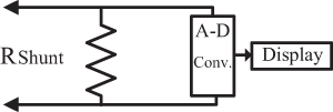
The intrusiveness of the measurement technique on the circuit can be further reduced by converting the meter into a digital display, as shown in Figure 2-29. The A-D converter can be much more sensitive than a meter coil and so can respond to a much smaller signal. Therefore, the shunt resistor can be very small. The smaller the shunt resistor, the less impact it will have on the circuit being tested.
2.5.3. Voltmeters
A small variation in the approaches shown in Figures 2-27 to 2-29 can turn our current meter into a voltmeter. Consider the circuit shown in Figure 2-30. A voltage is applied between the input and output. Resistors R1 and R2 form a voltage divider, with most of the voltage drop occurring across R1. Most of the current through the meter is shunted through R2, with a small amount of current passing through the meter movement itself. Switching circuits would switch various combinations of values for R1 and R2. With properly designed switching circuits and calibration, this technique can be used to measure voltage over a very wide range.
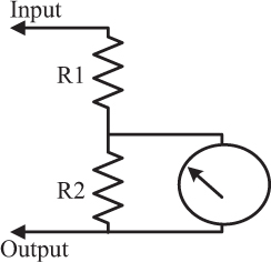
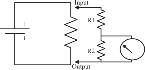
The voltmeter measurement does not require the current path to be broken (Figure 2-31). A voltmeter simply attaches to two points in a circuit and measures the voltage between those two points. Therefore, one way to measure the current through part of a circuit is to measure the voltage across a known resistance in the same part of the circuit and derive the current using Ohm’s Law (covered in Chapter 3). The analog voltmeter shown in Figure 2-31 could become a digital meter or oscilloscope simply by replacing the meter movement circuit with an A-D converter and digital display circuit as suggested in Figure 2-29.
An analog voltmeter presents a resistance to the circuit that is under test. Usually this resistance is part of the meter specification and is therefore known. For example, a reasonable portable voltmeter may have an input specification of something like 20,000 ohms per volt. This means that if there is a 5-volt range, the input resistance when used on that range will be 5 volts × 20,000 ohms/volt or 100,000 ohms (100K). In digital circuits this may present an unacceptable load on the circuit, changing the circuit being tested and therefore giving an invalid reading. Electronic voltmeters typically avoid this problem by having much higher input resistance and therefore much smaller signals at the point of measurement, but also having an internal amplifier to boost this signal before final measurement. It is this same reason that oscilloscopes also tend to present smaller loads to circuits under test.
2.5.4. AC Measurements
If an AC current were passed through the meter shown in Figure 2-25, the needle might never move. The polarity of the induced magnetic field would alternate with the frequency of the current and there would be no net torque in either direction. This is, or course, what would be expected if the average current were zero.
AC meters, therefore, usually have some sort of diode circuit allowing current to pass through the meter in one direction but not the other. One version of this is shown in Figure 2-32a. During the half-cycle when the AC signal is positive, current flows through the meter. During the other half-wave cycle, current is blocked by the diode and does not flow. The resulting waveform is called a half-wave (the diode acts as a half-wave rectifier).
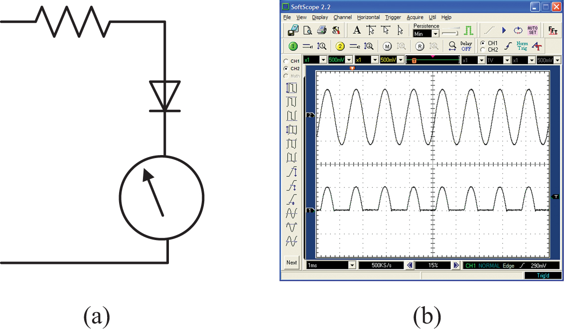
Typically, what we want the meter to indicate is the most useful measure—the RMS value of the waveform—which is 0.707 times the peak value. In this figure, what the meter will register is the average of the half-wave rectified sine wave—0.318 times the peak value. Thus, the scale on the meter face is typically calibrated so it displays 0.707 times the peak even though it is only measuring 0.318 times the peak value. Consequently, this type of meter only indicates the correct AC value when it is measuring a sine wave. Any other wave shape (with a different average value) will scale to an erroneous value! This is true of almost all AC meters. Only if the meter has a label saying it is a true RMS meter can you be confident that you are measuring the true RMS value of any waveform, regardless of its shape.
Historically, true RMS meters used some sort of power measurement to determine the RMS value of the signal being measured. The signal would be applied across a resistive transducer that would warm up in proportion to the power being applied. The change in temperature would be measured, converted into power, and then converted into an RMS value. Even though there are several possible sources of error with this technique, true RMS meters were actually surprisingly accurate.
In recent years, as the computational power of circuits increased and became more practical, meters could actually perform the RMS calculations in real time and display the results. Today, there are special integrated circuits dedicated to performing RMS calculations for voltmeters and current meters. Consequently, true, practical, and economical RMS meters are more common today than they were in the past.
2.5.5. Clamp-On Meters
Recall that the flow of electrons (current) along a wire produces a magnetic field around the wire. If you can measure the strength of the magnetic field, you can infer the magnitude of the current generating it. Clamp-on meters have a magnetically sensitive coil assembly that clamps around the wire carrying the current. Then, by measuring the strength of the field they can calculate the current through the wire (Figure 2-33).
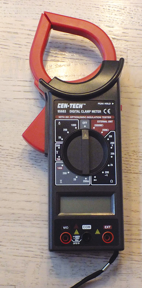
Clamp-on meters have significant benefits over other current meters: They are not intrusive, and they do not require that the circuit be broken in order to make the measurement. This is both a convenience issue and a safety issue, especially when measuring high currents in a high-voltage area. Their disadvantage is that they typically need access around the complete circumference of the single wire of interest. If two wires are enclosed by the clamp, the meter will read the net sum of the currents. If the two wires are the signal and its return (e.g., an ordinary extension cord), the meter will not read anything because the two wires contain currents that are equal and opposite. Thus, clamp-on meters are good for measuring current along an individual wire but are less valuable for measuring current along a printed circuit board trace. Some clamp-on meters are only accurate for sine wave signals, and some are true RMS versions.
2.5.6. Measurement Errors
Any measurement tool, of course, has some inherent level of accuracy. But beyond this, there is the additional problem that the process of measurement itself disturbs the effect being measured, which, therefore, might result in erroneous results.4 Users of tools must be aware of the possible effects their measurements might have on the circuit itself.
4. This is related to, but not exactly the same as, the “uncertainty principle” credited to Werner Heisenberg (1901–1976).
The primary source of possible error is caused by the fact that either (a) some current is diverted to the circuit doing the measurement or (b) the measurement circuit adds some impedance to the circuit being examined. In either case we say the measurement tool loads down the circuit.
For example, assume a voltmeter has an internal resistance of 20,000 ohms/volt and is used on a 5-volt scale. Thus, it acts as a 100,000-ohm (100K) resistor placed across the circuit under test. If the circuit under test also has an impedance of 100K, this load could change the circuit performance dramatically! But if the impedance of the circuit is only a few tens of ohms, there will probably be no error of measurement. The user must be aware of the nature of the circuit being measured so he or she can judge whether the tool being used will cause measurement errors.
Better portable meters have input impedances of around 20,000 ohms/volt. Cheaper meters can have input impedances as low as 2,000 ohms/volt, severely limiting where they can be used. Any meter should have its input impedance specification clearly visible on the meter face and in its documentation.
Powered meters (digital meters and oscilloscopes, for example) can have much higher input impedances. This is because they can deal with much smaller internal signals that are then amplified before measurement. Consequently, they load the circuits under test much less than portable meters typically do. Nevertheless, even these types of measurement tools can load the circuit under test. A major challenge for all test engineers is determining whether the measurement techniques themselves will cause changes in the circuit during test.
2.6. Thermal Noise and Current Thresholds
Absolute zero5 is the temperature at which all atomic motion stops. As elements warm, atomic and molecular motion increases. We know that elements pass through three states as temperatures rise: solid, liquid, and gaseous. Each is related to increased atomic and molecular motion.
5. Absolute zero temperature is –459° F, –273° C, or 0° K.
Electron motion is intimately related to temperature. The warmer the atom, the more motion that occurs within the atom, and the more electron motion there is. Now, if current is the flow of electrons and electrons are in motion because of temperature, an interesting question is “How do we tell the difference between motion related to an electronic signal and motion caused simply by temperature itself?”
Electrons that are in motion because of temperature cause an electronic signal that we call thermal noise. If you have a hi-fi system at home and turn the volume up very high when there is no signal present, you may hear something like a hiss from the speakers. A large component (if not all) of that hiss is caused by thermal noise. We sometimes call it white noise because it seems to be made up of all frequencies, just as white light is made up of all colors.
In general, we can’t tell the difference between electrons that are in motion because of a signal and those that are in motion because of thermal effects. Usually signals are very much larger than noise, and we talk about a signal-to-noise (S/N) ratio that compares the two. If the signal is much larger than the noise level (that is, many more electrons are moving because of the signal than are moving because of the noise), then it is easy to identify the signal component. If signal levels are very low, perhaps similar to the thermal noise levels, there are some things we might be able to do with signal coding, for example, to improve our ability to “pull” the signal out of the noise.
But the thermal noise level generally provides a threshold signal level below which we can no longer operate. A reasonably intuitive example is a telescope looking out at the stars. Light from the stars falling on some sort of photo detector creates a signal for us to process. If the light from the star cannot generate a signal stronger than the thermal noise level, we can’t see the star. This is what often limits the sensitivity of the telescope.
There are a few ways we can improve signal/noise levels. One is to code the signal. If we examine a certain time increment of the signal, thermal noise will be inherently random. If we have coded the signal, there will be a coherent signal we may be able to detect within the noise. Thus, coding can be used to allow communication at levels below the noise level.
A second possible solution is to preamplify the signal somehow before we begin to process it. This provides a possible “brute force” solution to the problem. And a third possibility is to cool the temperature of the electronics, thus lowering the thermal noise level. This is, in fact, one approach that has been used with telescopes. The initial circuits (the “front-end” circuitry) are placed in liquid nitrogen cooling tanks, driving down the noise level for that part of the circuit. Finally, it may be possible to buy special low-noise components for critical parts of a circuit. When all is said and done, however, thermal noise is the ultimate determinate of how low signal levels can be, and still be usefully detected and processed.