Columnstore structures that can improve performance of your reporting and analytic workloads
Memory-optimized tables that can improve your OLTP workloads with CRUD-like actions
Temporal tables that can preserve the entire history of the changes you made and enable you to perform historical and time travel analysis of data
Columnstore format
Rowstore format is the default storage format for tables in Azure SQL, and it is proven as an optimal structure for most general-purpose workloads. In rowstore format, the cell values belonging to a single row are physically placed close together in fixed-size 8KB structure called pages .1 This is a good solution if you should execute the queries that select or update the entire row or a set of rows. If you run the queries like SELECT * FROM <table> WHERE <condition>, where the <condition> predicate will select a single row or a small set of rows, the rowstore format is an excellent choice. Once the database engine locates the 8KB pages where the row(s) is placed, most of the data will be on that page and loaded with a single data page access.
In this type of analytical and reporting query, we need to access just two columns from all rows to calculate the result. Even in the presence of a Clustered Index , which would help to keep related data physically close to each other, a lot of resources will be put in loading data from unneeded columns: as obvious, this will have a negative impact on query performances.
It’s important to highlight that since a database is usually a very concurrent system, the fact that Azure SQL loads into memory data that it doesn’t need at all may not necessarily be a bad thing, as this will help other queries to have that data already in memory, and thus they will have better performance. As memory is a very limited resource, compared to disk space, it’s important to understand what are the typical workload patterns for your system, so that every recommendation or best practice can be put into your system perspective. Especially with databases that cannot be optimized only for reads or for writes, finding the best balance is the key goal for developers and DBAs.
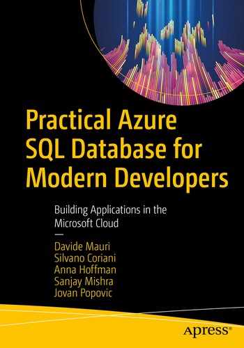
Rowstore format is optimal when a query needs to access all values from single or few rows (on left), while columnstore is optimal when the query accesses all values from single or few columns (on right)
In the rowstore format shown on the left side, a reporting query would need to go through all rows in the table, read every page, and take two out of ten columns in each row to calculate the result. This means that a query that uses two out of ten columns will roughly use only 20% of memory pages that need to read. If you have a table where you are using just the smaller columns for analysis, but you have big NVARCHAR columns in the row that will be discarded by the query, as they are not used in the specific query, the efficiency is even worse because NVARCHAR columns will occupy more space as their memory pages that must be fetched and discarded.
This might be a problem in memory caching architectures where underlying hardware takes the pages from the lower-level caches (or storage) to the higher-level memory caches because most of the data movement is in vain. Although that might look like a micro-optimization, you can see huge performance issues if you try to run these kind of queries on hundreds of thousands of rows already. Years of analysis and real-world experience show that the rowstore technology is not suitable for high-performance analytics and reporting.
Let’s now focus on the Columnstore representation of the rows on the right side of Figure 9-1. All values per column are physically grouped together. This means that the reporting query would easily pick up two columns that are necessary to compute the result and read only these values. Other values in the different columns are not used at all, and maybe they are even not in memory. Since the full-scan queries need to read all values from all or the majority of rows, the efficiency of memory read is close to 100%. All values within the same column are physically placed close to each other, and all of them will be read and used by the query. This significantly boosts performance of analytical queries. It's actually quite common to see performance improvements of 10 or 100 times the original times based on rowstore.
There is another optimization that can be leveraged in this case. All modern processors support SIMD (Single Instruction Multiple Data) operations that can extremely efficiently apply one operation on all elements in the memory array. If the storage organization enables us to provide a continuous array of cells that needs to be processed, SIMD instruction can apply a single operation on all values in the column segment. This is known as batch mode execution , and it is much more efficient than classic row-by-row processing.
NULL-Values elimination – If there is a large percentage of missing values in the cells, Columnstore will just avoid storing these rows.
Duplicate elimination – If a column has many identical values, Columnstore can record only one value and just mark the range of rows where this value occurs. This technique is also known as Run-Length Encoding.
Dictionary normalization – String and other discrete values are placed in internal key-value dictionaries per column segment. Keys are placed in column segments instead of actual values.
In addition to these strategies, entire segments can be compressed which can additionally save space. This is a common technique for the archival of data that is not commonly used but must stay in the database.
These are generic characteristics and advantages of columnstore format. In the following sections, you will learn about the specific implementation of Columnstore format in Azure SQL.
Columnstore in Azure SQL
Azure SQL doesn't use the classic Columnstore organization described in the previous section. In theory, we could create large column segments where each one would contain all values from a single table column and compress it. However, on any update we would need to decompress the entire column segment to insert, update, or delete a single value and then compress it again. To avoid this overhead, it might be better to split the unique column area into multiple column segments and perform the needed operations only on the segments that contain cells that need to be updated. In addition, most of the queries would not need to scan all rows, so most of the cells that would be decompressed would not be used. If we split a column into multiple column segments, maybe we can pick only the segments that are needed in query. The idea is very similar to a partitioning technique, but just applied within the column segment and in a totally transparent way for the user.
Column segments do not span over the entire table. Azure SQL will divide table rows in the groups up to 1 million rows. These row groups are organized in Columnstore format, and every column segment has up to one million rows’ values.
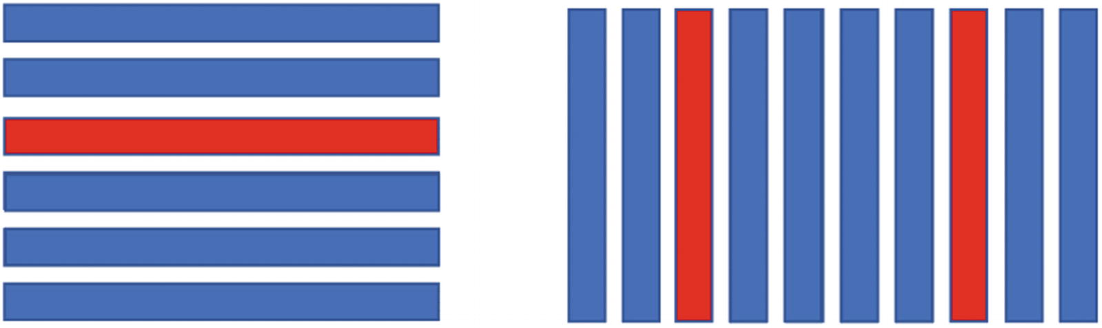
All new rows are inserted in a buffer row group organized using the rowstore format. Rowstore format is the perfect choice for row-oriented operation, so it makes sense to use it as an area for inserting new rows. These row groups are called Deltastore. Once these row groups reach one million records, they are transformed and compressed – transparently and in the background – into columnstore format.
Columnstore structures have a compressed area in Columnstore format and input area in rowstore format (Delta)
Compressed area containing many columnstore organized groups of rows where column segments in row groups are highly compressed. Ideally, all row groups would be compressed in this area.
Deltastore area containing one or more rowstore organized groups of rows. This is the temporary buffer area with the rows that are waiting to be compressed and moved to the compressed area.
The compressed area should contain more than 95% of data, and compressed data should not be changed. It’s undesirable to modify data in the compressed area because Azure SQL would need to decompress all values in the segment to update just one and then compress everything again.2
There is another area in the Columnstore structure called Deltastore. Deltastore contains a smaller set of row groups organized in a classic rowstore format (or Hobit described in the previous chapter). The main purpose of this area is buffering the new inputs and changes before they get compressed. Splitting every new row into each column and re-distributing values into corresponding column segments would be an inefficient strategy to insert data. Therefore, all new rows are inserted in the rowstore delta area where they reside until the row group gets up to one million rows. Once the row group in the delta store is filled, it is closed for new changes, and a background process will start converting this row group into Columnstore format and moving it into the compressed area. The goal is to move as much as possible row groups from delta storage into compressed storage, and delta storage should contain less than 5% of rows.
In theory, we could have only one row group in the delta store. However, one row group might affect concurrency because one transaction that is inserting data might lock the row group and other requests that are trying to insert data would need to wait until the first one releases the lock. Therefore, the Columnstore structure creates new row groups to facilitate concurrent inserts.
Updating values in Columnstore
As already mentioned, updating compressed Columnstore data is not a desired action. Columnstore format is not read only, but updates have a bigger penalty compared to classical rowstore. Azure SQL has some enhancements that optimize updates of compressed data.
If you insert a smaller amount of (less than 102,400) rows, all rows will land into some Delta row group.
If you insert more than 102,400 rows using single BULK INSERT or SELECT INTO statements, Azure SQL will stream these values directly into new compressed row groups.
Another problem that needs to be solved is how to efficiently delete rows from a columnstore. Unpacking 1,000,000 rows to delete one and then compress 999,999 is not a desirable technique. Azure SQL uses so-called Delete indexes and Delete bitmaps to “virtually” delete the rows. Whenever you need to delete a row from a compressed row group, Azure SQL will just “mark position” of this row as deleted. Whenever you read the rows from compressed column segments, Azure SQL will just ignore the rows marked as deleted at runtime. This way, the query that is reading data from the column segments is getting only existing rows and doesn’t need to be aware that the deleted rows are transparently excluded once the row groups are decompressed.
There is only one operation left to be dealt with now: updating data. This is the most complex operation, as Azure SQL cannot just inject an updated value into an existing, highly compressed column segment without decompressing and compressing again everything else also. For this reason, every row update is represented as a combination of delete and insert operations. Old values of the row in the compressed row group are marked as deleted, and the new value is inserted in the delta store.
Marking deleted rows and representing updates as a pair of delete and insert operations are used only if the affected row is in a compressed area. If the row is in the Delta store, it will be updated or deleted as any other row in regular Hobits.
Querying Columnstore structure
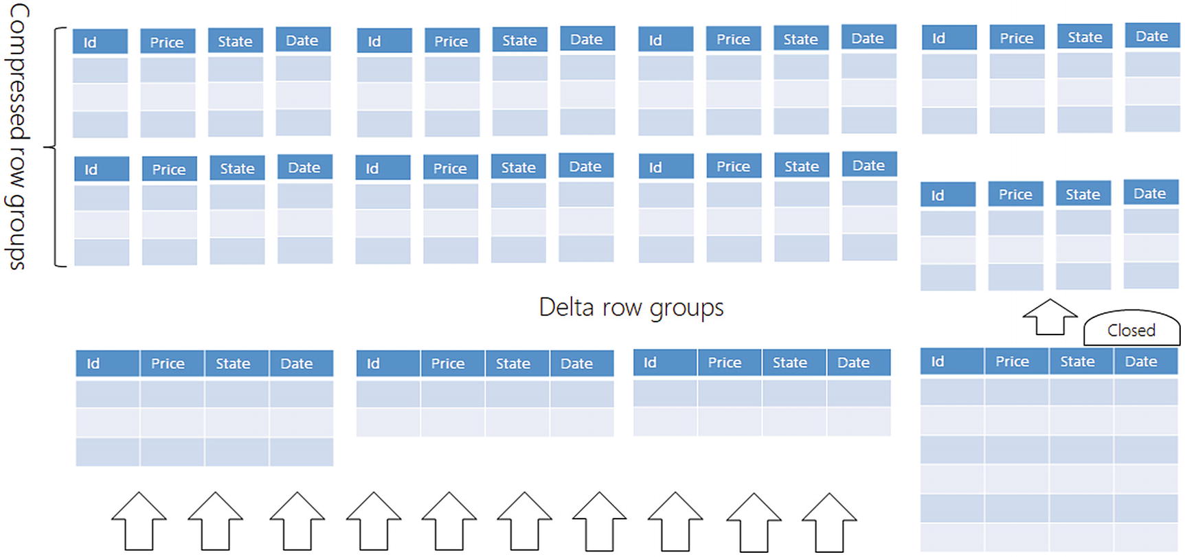
Let’s imagine that the table in the example has six compressed row groups with five columns (five column segments per each row group).
Column segments that belong to the columns that are not used in the query are ignored.
Column segments that don’t have the values required in the query are ignored.
Columnstore will discard column segments that are not needed for the query (red) and column segments that don’t contain data required by query (orange)
The columns Id, Date, and Tax are not used in the query, so Azure SQL will not even load them into the memory if they are still on disk. This way, we are reducing the required IO and memory footprint to 40% because three of five column segments are ignored.
Each column segment contains some statistics about the values in the segment (e.g., min-max values). Azure SQL knows what column segments contain the values Available and In Stock. Let’s imagine that these values appear only in three row groups out of six row groups. Azure SQL will discard State column segments that don’t contain the values used in the query and related Price column segment from the same row groups. This way, Azure SQL will discard another half of the data without even starting the query. These optimizations have a huge effect if most of the data is stored in compressed column segments and not in Deltastore.
Imagine that the dataset used in this example initially had 100GB. Under assumption that columnstore structure can have 10x compression and that column segment elimination can discard 80% of data before query starts, we are getting 2GB that should be processed instead of full table scan. This is a huge reduction of required IO and memory for the query that can boost performance up to 50x.
Another important optimization is batch query processing. Azure SQL will leverage underlying hardware SIMD instructions and apply a small number of operations on large vectors of data. The vectors of data are column segments containing the continuous range of values. This hardware acceleration in a batch mode processing significantly improves performance of the queries and is completely transparent to the query and thus to the application using it. The query will just run faster.
Clustered Columnstore indexes
We are using CCI to store highly compressed data with dominant read and massive (bulk load) insert workload patterns. This workload pattern is very common in data warehouses, and this is the reason why CCI is a very common structure in modern data warehousing scenarios. However, CCI is applicable in any scenario where you are going to append and analyze data, such as IoT scenarios.
CCI boosts performance of reporting and analytic queries using compression and batch mode execution, which are the primary benefits of Columnstore format.
CCI reorganize operation is a lightweight non-blocking operation that will merge and compress open delta row groups without major impact on your workload.
Nonclustered Columnstore indexes
Classic rowstore table with additional Columnstore index (NCCI) built on top of the tree columns from this table
The main purpose of NCCI is to optimize analytical and reporting queries on the subset of columns in the existing rowstore tables without changing the original table structure.
If you run some query that selects a single row or small set of rows, Azure SQL will use the underlying rowstore table. Database will leverage index seek or range scan operations that are the perfect fit for this scenario.
If you run some report that scans the entire table and aggregates data, Azure SQL will read information from NCCI index, leveraging column segment elimination and batch mode execution to quickly return process all table.
Any update, delete, or insert will immediately end up in the underlying rowstore table, and NCCI will be updated via Deltastore. This double update might slow down your transactional workload, but this should be acceptable if you need to make a trade-off between boosting reporting capabilities on a table and speed of transactional statements.
Memory-optimized tables
Azure SQL has memory-optimized tables that might extremely improve performance and the scalability of your OLTP workload. The main purpose of memory-optimized tables is to improve CRUD-like operations like selecting a few rows or updating or deleting existing rows.
Some people assume that keeping the rows always in memory is the key factor that improves performance. However, this is a naïve assumption that in many cases is far from the real reason.
Azure SQL always works with rows that are placed in memory. It has an excellent mechanism for caching data in memory (called Buffer Pool), picking the most important data that should be fetched from disk, and smartly evicting the rows that should not be needed in the near future to make space for more likely-to-be-used rows. If your database is smaller than memory, all rows will probably be in RAM, so you will already have an “in-memory database.” So, the question is what kind of additional “memory optimization” do we get with the memory-optimized tables?
As mentioned before, all data stored in the database is memorized on disk using 8KB data structures called pages. A 10GB uncompressed database will have something like a million data pages at minimum.
Every time a row is accessed, the related data page is loaded in memory. Azure SQL will try to keep as many data pages in memory as possible. This memory section is called the Buffer Pool.
Buffer pool cannot cache all data if the database is bigger than the available memory, and thus the pages must be fetched from disk and persisted back to disk if they are changed. Every page is read or written as an atomic 8KB unit. Sometimes, databases can read bigger chunks of disk with a single IO operation (so-called read-ahead operations) to optimize IO performances.
The most expensive operation in a query is transferring 8KB pages between memory and disk.
Data transfer between memory and disk should be minimized. The database engine should do its best to prevent unnecessary IO interactions.
Pessimistic where we are blocking other threads that would like to access rows already modified by another thread, until the modifying thread decides to save or reject the changes.
Optimistic where we let other threads access the original version of the modified rows. We need to make a copy of the rows that will then be a “private version” available only to the current thread, while others are accessing the original row.
Ideally, we should be optimists because a pessimistic approach blocks other threads, which mean less performances, concurrency, and scalability. But we need to be aware of pros and cons of both approaches.
A story about optimistic concurrency

Creating new versions of updated rows for every transaction that makes the changes
Once Tx1 commits the changes on row 1, the easiest thing that Azure SQL can do is to declare the old data page as invalid and use the new page. Because it would be hard to copy part of the page back to the original 8KB page. Tx2, which was also working on a private copy of row 1, would not be able to commit its own row because it updated a version that is not valid anymore. Once Tx2 tries to commit the change, it will be rolled back and would need to retry the operation with latest valid data. This might be expected because both transactions tried to update rows without locking it exclusively. If there is a collision, retry is the only solution. In addition to this, there is also another, maybe unexpected, side effect. Tx3 would not be able to commit its own row changes, even if those were done on a row different than row 1, and thus didn’t clash with the row 1 updated by Tx1. Since the binary content is changed and maybe the page is split into two new pages, Azure SQL cannot easily get the binary content of the changed row from a new valid page. Therefore, this transaction will be rolled back too.
In addition, there is a performance impact of creating new pages with temporary rows. Azure SQL has a background process called “Checkpoint writer” that saves modified memory pages to underlying storage. If we get a lot of temporary pages, they would be saved on disk, and then after rollback, original content must be saved again. In this case, temporary generated pages would cause more damage and we might want to prevent this.
Should we be pessimists?
Since the 8KB page is the main unit of data transfer, transactions that update the rows might take a lock on the entire page and prevent others making changes that would very likely be rolled back and cause additional IO. Locking mechanisms are pessimistic approaches that help to prevent damage, due to race conditions , that concurrent queries might cause on a single page.
As you learned in Chapter 7, usually the database prevents the risk of having too many IO operations by using pessimistic concurrency control. Every transaction is taking locks or latches (latch is just a more lightweight version of lock) to ensure that one version of a potentially shared row or data page is exclusively dedicated to the thread that is modifying it. Other threads that want to change data on the same page are temporarily blocked by row locks or page latches while another thread is modifying it. Threads cannot modify the same rows and they are blocked. This way, we avoid a need to create new pages and cause additional IO, but we are decreasing concurrency and affecting performance.
Now, let’s imagine that we can forget about disk IO and that we don’t have 8KB pages that would need to be persisted even for the temporary changes. We could use high, optimistic concurrency that uses just inexpensive memory copy operations and easily generate new row versions. This is possible only if we can be sure that table data will be placed in memory without data transfer between buffer pool and disk storage and that there is no 8KB container that causes dependency between rows. Memory-optimized tables provide these guarantees.
Memory-optimized tables are the tables where we know that data will be in memory so we can apply optimistic concurrency and allow a large number of concurrent updates. This is the main advantage of memory-optimized technology and the key differentiator compared to classic Hobits.
Memory-optimized tables
The only change that you need to do is to add a WITH clause with the property MEMORY_OPTIMIZED=ON. With this property, data rows are always kept in memory, data pages are not used anymore, and memory-optimized features such as optimistic concurrency are enabled on the table data.
Memory-optimized non-durable schema-only tables. These tables are very similar to temporary tables. The table schema will be preserved after restarts or potential system crashes. Azure SQL will re-create the table structure after restart, but it will not preserve the content. The main purpose of these tables is caching scenarios (like ASP.NET session state), being an intermediate store for complex data processing and fast loading of data (so-called staging tables).
Memory-optimized durable tables where both schema and data are preserved even after process crash or failover. Azure SQL will ensure that a minimal set of information is sent to log and persisted so data will survive system crashes. These tables are logically equivalents of classic tables with memory-optimized enhancements and used to improve performance of the existing rowstore tables.
Memory-optimized Columnstore tables are a combination of Columnstore structures and memory-optimized tables. The main scenario is a combination of analytic and transactional workloads (OLTP) on the same table. This combination is known as Hybrid Transactional-Analytical Processing (HTAP).
If you are wondering why you may want to use Azure SQL Memory-Optimized tables to create a caching solution, since there are other specific solutions like Redis or Cosmos DB that are usually better suited for caching, you should keep in mind that one of the best advices in software development is keeping things simple. If you are already using Azure SQL in your project, the option to create a custom transactional caching mechanism right into the database without having to resort to another technology can simplify your solution a lot (and also decrease maintenance costs, as you don’t have to learn and maintain another technology). In addition to that, Memory-Optimized table offers a deep integration with all other features of Azure SQL. For example, you can create a secured caching solution by using Row-Level Security with Memory-Optimized tables.
DURABILITY=SCHEMA_ONLY defined non-durable table where only table structure will be re-created if Azure SQL Database restarts.
DURABILITY=SCHEMA_AND_DATA defines a durable table where both table structure and data will survive failover or crash.
Columnstore memory-optimized tables combine best from both worlds – extremely fast analytic and compression of data that can fit into memory and highly-concurrent and extremely fact ingestion and updates of data provided by memory-optimized tables. The only risk here is the amount of data that you can process. Classic Columnstore indexes analyze all data in memory; however, it lets you keep column segments on disk if they cannot fit into the memory. Memory-optimized Columnstore requires all data to reside in memory. Since Azure SQL reserves ~60% of available memory to memory-optimized data, you need to be sure that your data can fit. Since we are talking about large amounts of data in a Columnstore analytic scenario, if you are not sure that your data can fit into memory, use disk-based tables.
For these reasons, Memory-Optimized Clustered Columnstore Indexes cover a niche scenario. In fact, using classic rowstore tables with NCCI indexes for HTAP scenarios is the general approach on average, and Memory-Optimized Clustered Columnstore Indexes are used only on very performance-intensive workloads. For example, if you need to be able to handle up to 5 million of rows per second, like described in the article “Scaling up an IoT workload using an M-series Azure SQL database” referenced in the last section of this chapter, you will needed Memory-Optimized Clustered Columnstore Indexes for sure.
While we are talking about memory-optimized storage, we cannot separate this discussion from indexing. In-memory rows are objects scattered in memory space and need some structure that will bind them together. These structures are the indexes. Whenever you create memory-optimized, you need to have at least one index.
NONCLUSTERED HASH index is an in-memory hash table that uses column values as keys (EmpID in this case) and contains a list of pointers to the actual rows in the table. Every hash table consists of a fixed number of slots (hash buckets) with an array of pointers to the actual rows. Row pointers with the same hash values are linked into the list that represents its own hash bucket.
The bucket count must be specified at index creation time and impact the length of the pointer list in every bucket. The ratio of distinct key values and the number of hash buckets would represent the expected average bucket link list length. Longer lists imply more operations to find the row based on key.
The bucket count should be between one and two times the number of distinct values in the index key. In practice, it is hard to estimate the number of distinct values in a column; however, you will get good performance if the BUCKET_COUNT value is within ten times the actual number of values in the indexed column. Note that overestimating is generally better than underestimating. If you find a bad ratio after some time, you can always rebuild the index with new bucket count.
Accessing memory-optimized tables
Another advantage of memory-optimized tables is the fact that they can be accessed like any other classic table. You can use the same Transact-SQL queries to join memory-optimized tables, Columnstore table, and classic Hobits.
Interoperability between the different features such as Columnstore, memory-optimized tables, JSON, and graphs is one of the core value propositions of Azure SQL. Any feature that is specific or optimized for some scenario will have the same or similar access methods.
Memory-optimized tables use optimistic concurrency control that quickly creates a new version of row whenever some transaction updates it. This way, transactions that update data are getting their own private version of row without getting blocked by readers or blocking other writers.
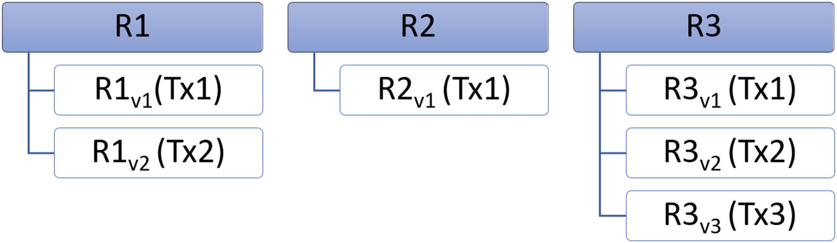
New row version is created whenever some transaction updates the row
This row versioning has some implications on some transaction isolation levels used in Azure SQL. Disk-based tables enable you to read the temporary uncommitted values of the rows if you are sure that this is what you want and bypass the locks. This is not possible in memory-optimized tables because there can be multiple uncommitted copies of the same row and Azure SQL doesn't know which of these versions you would like to use.
Also reading committed rows is not as easy as with regular tables. If you would like to read committed rows, your transaction would always need to check if the current row is really the latest or if there is some transaction that committed a new public version. This might be huge performance overhead that you surely want to avoid.
The solution is to use a committed version of a row at the time of beginning your transaction, which looks like a snapshot of table data. The transaction isolation level that works with snapshot of data at the beginning of a transaction is called SNAPSHOT isolation level.
WITH(SNAPSHOT) hint instructs Azure SQL to interpret the values in the table as a snapshot of the data state at the time of execution. This isolation level ignores the changes that might occur in the meantime. This hint will prevent the error with code 41368 in other isolation modes.
If you properly set up transaction isolation level, there are no big limitations in DML statements that you can use to query memory-optimized tables.
Natively compiled code
Azure SQL interprets the batches of T-SQL code that you use to work with data. This means that the query batches (one or more T-SQL statements) are parsed, then every query in the batch is compiled into an Execution Plan, which is broken down into operators (e.g., scan, join, sort), and the operators are executed to fetch or update the rows. This strategy of query processing might be a big bottleneck while working with memory-optimized data. Although you have data available in memory and minimal locks, chains of operators will still use classic mechanisms to fetch row by row and process it.
Azure SQL enables you to use natively compiled modules to improve performance of your T-SQL code. You can imagine natively compiled modules in Azure SQL Database like customized C programs – yes, that’s right, C programs! – that process your data. Transact-SQL code will be pre-compiled into native .dll – dynamically linked libraries – and then executed by the Azure SQL engine to operate on data. Imagine that you have an API that accesses memory rows as lists or iterators and that you want to create a C code that iterates through the rows and applies some processing (similar to LINQ queries in .NET technology). This would probably be the faster way to work with data, but it might be hard to write this.
As writing C modules to manipulate data is not an easy task, in order to remove complexity and still enable you to boost performance, Azure SQL Database allows you to declaratively write standard T-SQL code that accesses rows in memory-optimized tables. This T-SQL code will be translated into the equivalent C code that accesses table rows using internal API and compiled into native executable that will be executed in Azure SQL database process. This way, you are still expressing what you want to do using T-SQL code, and Azure SQL Database handles all complexity of accessing API via C language, unlocking extreme performances.
Azure SQL enables you to write SQL procedures, functions, and Triggers that will be compiled into native executables. Natively compiled code might be orders of magnitude faster than classic counterparts. The only limitation is that they can access only memory-optimized tables and use a subset of T-SQL language.
Any T-SQL code that is placed in the body of this procedure will be parsed, and the equivalent C code will be generated and compiled into a small dynamically linked library (.dll) file.
WITH clause that defines procedure properties such as marking procedure as natively compiled and specifying schema binding. Schema binding means that the tables referenced by the Stored Procedure cannot be altered as long as the procedure exists. These are the only required options, but you can also specify others such as EXECUTE AS and so on.
ATOMIC block representing a unit of work that will be either processed or canceled. In the atomic block, you need to specify options such as isolation level or language because these settings will be compiled into the dynamically linked library.
We have seen in Chapter 8 that Azure SQL does not use native JSON type. JSON is stored as a NVARCHAR string that should be parsed at the query time. With a natively compiled function, we can explicitly define parsing rules that should be used and create a native built-in custom JSON parser.
Accessing memory-optimized tables using natively compiled code is the recommended way as it provides the best performance and scalability possible.
Temporal tables
Error correction – Someone accidentally changed or deleted a row in a table, and you need to correct or revert this change.
Historical analysis – You need to analyze the changes that are made in the table over time.
Auditing – You need to find out who changed the values, when, and what was changed.

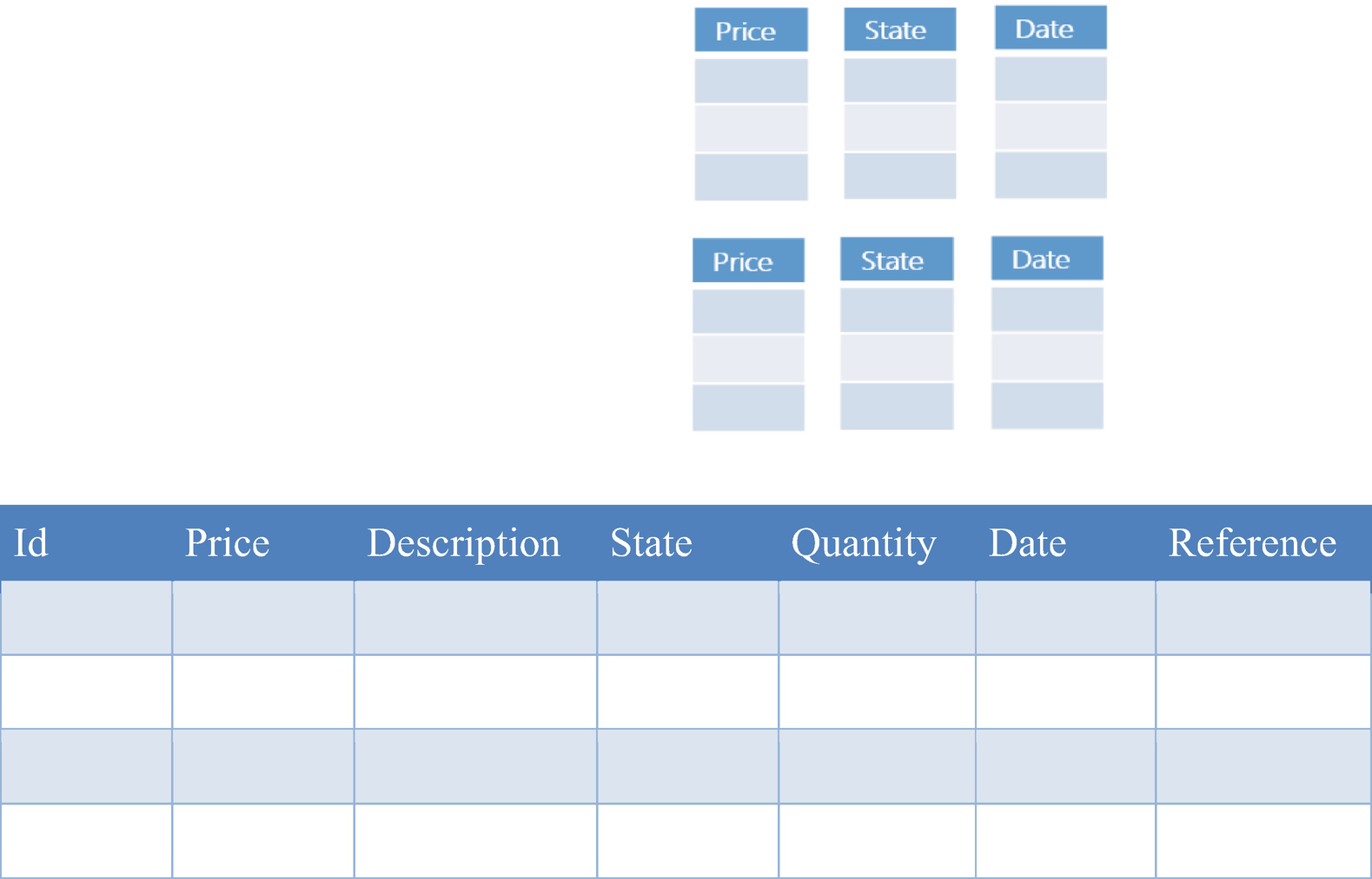
Temporal table automatically sends the row that will be updated or deleted into a separate history table
The queries that just insert or select data will work only with the main temporal table, where the current version of data is stored, and they would not affect the history table. Temporal tables modify behavior or the queries that update or delete data and silently send current row values to the history table before they are updated in the main table. This is completely transparent, and you can keep using the standard T-SQL queries to access data.
Moving old rows in the history table before they are changed is one of the most common scenarios for Triggers. Temporal tables provide native support for this behavior by automatically moving rows. The method used in temporal tables should be much faster than equivalent Triggers in most of the cases.
Querying temporal data
Automatic movement of old rows from the temporal to history table is important, but not the only benefit that you are getting from temporal tables. Even if you have all required row versions in the history table along with their validity range, querying historical data is still not easy. If you want to see how tables looked at some point in time in history, you would need to take some old row values from history but also some rows from the main table because they might be still valid at current time.
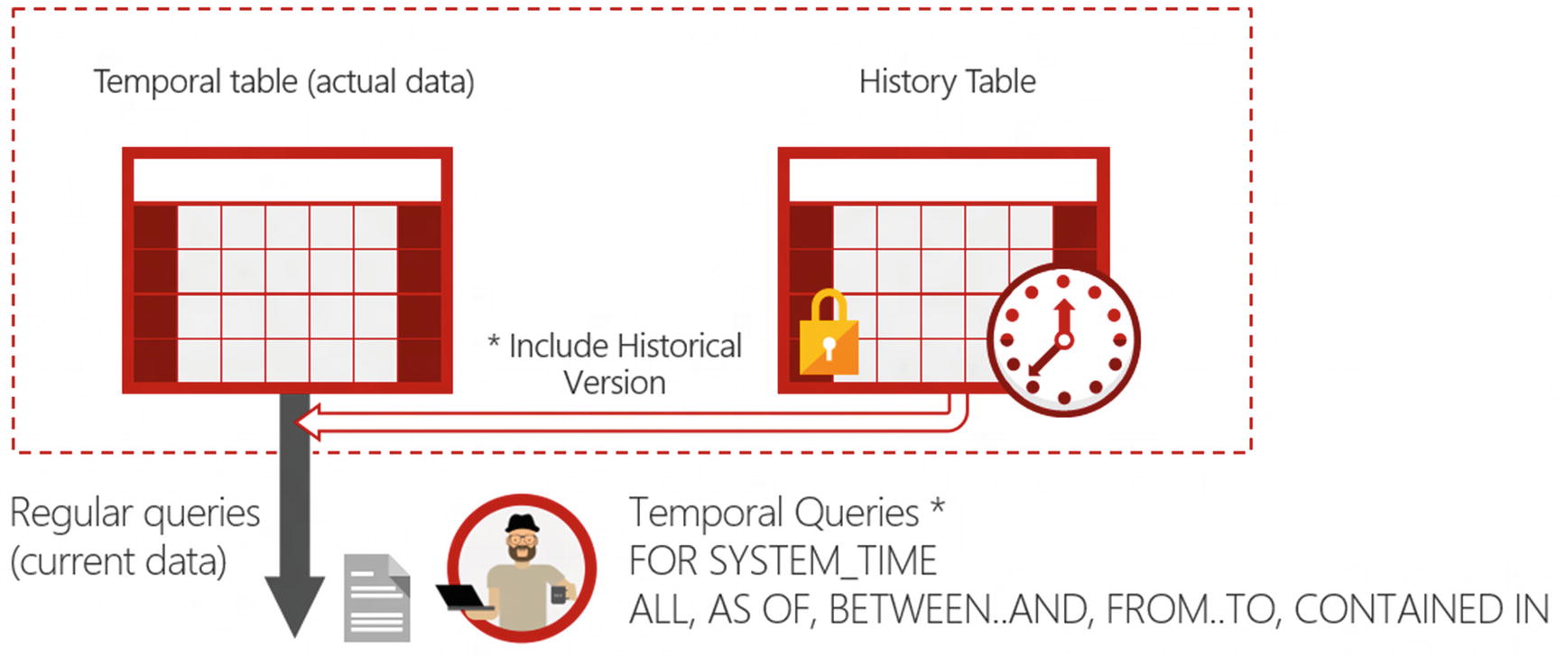
Temporal table enables you to fetch historical data for temporal queries
FOR SYSTEM_TIME AS OF <datetime> – The query will read the content of the table at the specified datetime in the past.
FOR SYSTEM_TIME ALL – The query will read all rows that existed at any point in time in the past.
More are available and you can find more details on those in the referenced resources at the end of this chapter. Depending on the temporal operator and the values provided to the operator, Azure SQL will decide if data must be read from the main table or from both tables and create the right plan that will fetch and merge resultsets from both tables.
Azure SQL will compare the datetime value of @asOf variable with the dates when the Employee row was changed. If the last change was before that date, it will fetch data from the main table. Otherwise, it will find a row in history that was valid in the specified time.
We are updating a row in the Employee table with a specified Employee primary key value (@EmployeeID). We are joining the row with the version of the row with the same primary key value at the specified time (@asOf) using FOR SYSTEM_TIME AS OF clause. Then, we are just overwriting the values in the recent version with the values from the valid version. Note that the faulty values are not overwritten without trace. When the error is corrected, the wrong values are moved into the History table, and you can track when they were corrected and what were the errors. The History table is the source of truth where you can find information about any change that was made on the temporal table.
Configuring temporal tables
The table that contains current data should be implemented as a memory-optimized schema and data table, if possible.
History table should be implemented with a Clustered Columnstore index.
If you are using the Business Critical service tier, a memory-optimized table will provide you the best performance in the workloads that insert, update, and delete data, which is the main scenario for tables with the current rows. You should not use memory-optimized tables if you think that all rows cannot fit into the memory, as having all rows in memory is a requirement for memory-optimized tables, as explained in earlier sections.
Columnstore format is the optimal solution for the history table because you can have many column cells with the same values. In many cases, you will update just a few columns leaving other cells unchanged. Temporal tables will physically copy the entire previous row to the history table, meaning that unchanged cells will have the same values in different row versions in history. Columnstore format has the most efficient compression if it can replace a set of cells with the same values with a single marker describing the range of rows where this value appears. In this scenario, the Clustered Columnstore index created on the history table could provide extreme compression and improved history analysis performance on the temporal table.
Clustered Columnstore indexes will provide high compression and improve analytic capabilities when the query scans large amounts of history data. Nonclustered indexes on range columns and primary key would be very helpful to boost the performance of those queries that are accessing values of some rows at a specified point in time in history (e.g., using FOR SYSTEM_TIME AS OF clause). Depending on the types of the historical queries that you are running, you might want to add the first, the second, or both indexes.
This database-level option enables you to switch on or off retention policy for all tables in the database.
If you want to know more
Columnstore indexes: Overview – https://docs.microsoft.com/sql/relational-databases/indexes/columnstore-indexes-overview
Columnstore indexes - Data loading guidance – https://docs.microsoft.com/sql/relational-databases/indexes/columnstore-indexes-data-loading-guidance
Get started with Columnstore for real-time operational analytics – https://docs.microsoft.com/sql/relational-databases/indexes/get-started-with-columnstore-for-real-time-operational-analytics
Niko Neugebauer Blog Columnstore Series – www.nikoport.com/columnstore/
In-Memory OLTP and Memory-Optimization – https://docs.microsoft.com/sql/relational-databases/in-memory-oltp/in-memory-oltp-in-memory-optimization
Memory-Optimized tempdb Metadata – https://docs.microsoft.com/sql/relational-databases/databases/tempdb-database#memory-optimized-tempdb-metadata
Optimize JSON processing with in-memory OLTP – https://docs.microsoft.com/sql/relational-databases/json/optimize-json-processing-with-in-memory-oltp
Temporal Tables – https://docs.microsoft.com/sql/relational-databases/tables/temporal-tables
Querying data in a system-versioned temporal table – https://docs.microsoft.com/sql/relational-databases/tables/querying-data-in-a-system-versioned-temporal-table
Scaling up an IoT workload using an M-series Azure SQL database – https://techcommunity.microsoft.com/t5/azure-sql-database/scaling-up-an-iot-workload-using-an-m-series-azure-sql-database/ba-p/1106271#