Rather than recklessly diving right into drawing, it would be helpful to first understand the canvas. In Chapter 2, the Display object was introduced. This represents the window in which the image is displayed. The SimpleCV framework currently only supports a single display window at a time and only one image can be displayed in that window. In most cases, the display is automatically created based on the size of the image to be displayed. However, if the display is manually initialized, the image will be automatically scaled or padded to fit into the display.

from SimpleCV import Display, Camera, Image

display = Display(resolution = (800, 400))  

cam = Camera(0, {'width': 320, 'height': 240})  

img = cam.getImage()

img.save(display)  

# Should print: (320, 240)
print img.size()

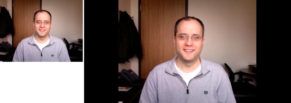
Figure 7-1. Left: The image as captured by the camera; Right: The image was scaled up so that it vertically filled the display, and then padding is added to the right and left to horizontally fill the display

Notice the result in this case. The window remains 800×400. The image is scaled up so that the height now matches the 400 pixels of the window. Then padding is added to the left and right sides. The effect is similar to the adaptiveScale() function. The original image size is not altered. You can see this effect in Figure 7-1. It remains 320×240 as is shown in the print statement, but it is scaled for display.

Images can also be divided into layers. Layers act like multiple images that sit on top of each other. The order of the layers is important. Items on the top layer cover items in the same area on the layer beneath it. Otherwise, if there is nothing covering them, the items from the lower layers will show through. Although all processing could be done on a single layer of an image, multiple layers can simplify processing. For example, the original image can sit on the bottom layer, and then lines drawn around the edges of objects can appear on the next layer up. Then, text describing the object can sit on the top layer. This preserves the original image while ensuring that the drawings and markup appear to the end user.

With the preliminaries aside, it is time to start drawing. Layers are implemented in the DrawingLayer class. For those who have previous experience working with PyGame, a DrawingLayer is a wrapper around PyGame’s Surface class. This class has features for drawing text, managing fonts, drawing shapes, and generally marking up an image. Remember that one key advantage is that this all occurs on a layer above the main image, leaving the original image intact. This enables convenient markup while preserving the image for analysis.

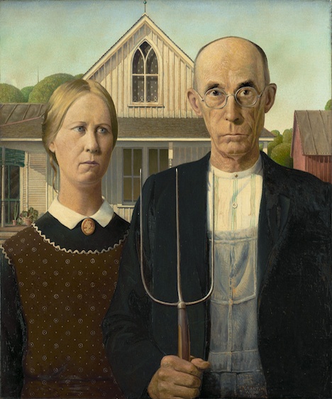
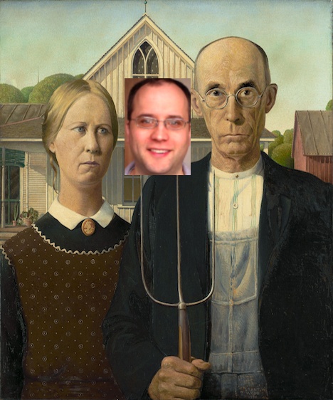
One of the easiest examples of using a layer is to draw one image on top of another. The following example demonstrates how to insert yourself into the classic American Gothic painting (by Grant Wood), as demonstrated in Figure 7-2.

Figure 7-2. American Gothic by Grant Wood

from SimpleCV import Image

head = Image('head.png')

amgothic = Image('amgothic.png')

amgothic.dl().blit(head, (175, 110))  

amgothic.show()

The resulting program adds a third person into the image, as demonstrated in Figure 7-3.

Figure 7-3. Three’s a crowd

A lot of stuff is happening under the hood in the previous example. To look at this in more detail, consider the following example, which works with the underlying layers:

from SimpleCV import Image, DrawingLayer

amgothic = Image('amgothic.png')

size = amgothic.size()

# Prints the image size: (468, 562)
print size

# Prints something like: [<SimpleCV.DrawingLayer object size (468, 562)>]
print amgothic.layers()  

layer1 = DrawingLayer(size)  

amgothic.addDrawingLayer(layer1)  

# Prints information for two DrawingLayer objects
print amgothic.layers()

The above code essentially manually does everything that was done earlier with background.dl(). Obviously this is more complex, but it shows in more detail how to work with layers:

The above process—creating a drawing layer and then adding it to an image—can be repeated over and over again. The layer added in the example above does not do anything yet. The next example shows how to get access to the layers so that they can be manipulated.

# This code is a continuation of the previous block of example code

# Outputs: 2
print len(amgothic.layers())

drawing = amgothic.getDrawingLayer()  

drawing = amgothic.getDrawingLayer(1)  

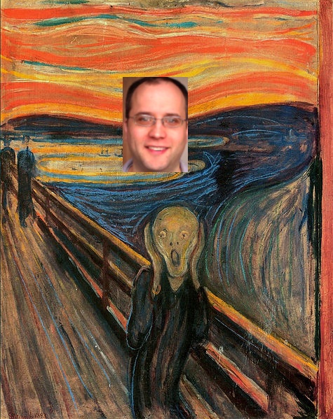
In the previous examples, a drawing layer is first created, and then that drawing layer is added to an image. The layer is not actually fixed to the image. Instead, a layer from one image can actually be applied to another image. The following example builds off the first example in this chapter, where a face was placed on an image. This re-extracts the face from a layer, and then copies that whole layer to a new image.

from SimpleCV import Image, DrawingLayer

head = Image('head.png')

amgothic = Image('amgothic.png')

scream = Image('scream.png')

amgothic.dl().blit(head, (175, 110))  

layer = amgothic.getDrawingLayer()  

scream.addDrawingLayer(layer)  

scream.show()

The resulting image will look like Figure 7-4.

Figure 7-4. A face that would make anyone want to scream

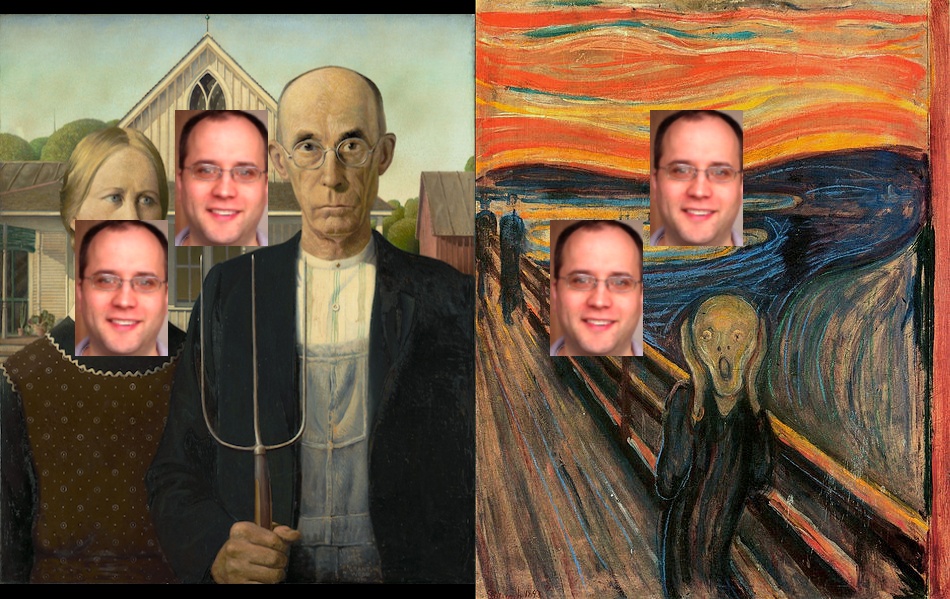
As demonstrated above, when copying a layer between images, the same layer is actually shown on both images. In other words, when a layer is modified, the resulting change appears on both images.

# This is a continuation of the previous block of example code

print amgothic._mLayers  
print scream._mLayers

layer.blit(head, (75, 220))  

amgothic.show()  
scream.show()

Notice that now the change appears on both images, as demonstrated in Figure 7-5.

Figure 7-5. The picture was added to the layer, making it appear on both images

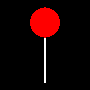
The SimpleCV framework includes tools to draw several basic shapes such as lines, bezier curves, circles, ellipses, squares, and polygons. To demonstrate the true power of the drawing engine, Figure 7-6 is a rendering of a lollipop (there is a reason we did not go to art school):

from SimpleCV import Image, Color

img = Image((300,300))  

img.dl().circle((150, 75), 50, Color.RED, filled = True)  

img.dl().line((150, 125), (150, 275), Color.WHITE, width = 5)  

img.show()

Figure 7-6. An example lollipop using the circle and line commands

Most of the time, rather than drawing on a blank image, we want to mark up existing data. Here, we show how to mark up the camera feed to make it easier to find and calibrate the center by adding markup similar to a scope (see Figure 7-7):

from SimpleCV import Camera, Color, Display

cam = Camera()
size = cam.getImage().size()
disp = Display(size)

center = (size[0] /2, size[1] / 2)

while disp.isNotDone():
     img = cam.getImage()

     # Draws the inside circle
     img.dl().circle(center, 50, Color.BLACK, width = 3)  

     # Draws the outside circle
     img.dl().circle(center, 200, Color.BLACK, width = 6)  

     # Draw the radiating lines
     img.dl().line((center[0], center[1] - 50), (center[0], 0),
          Color.BLACK, width = 2)
     img.dl().line((center[0], center[1] + 50), (center[0], size[1]),
          Color.BLACK, width = 2)
     img.dl().line((center[0] - 50, center[1]), (0, center[1]),
          Color.BLACK, width = 2)
     img.dl().line((center[0] + 50, center[1]), (size[0], center[1]),
          Color.BLACK, width = 2)

     img.save(disp)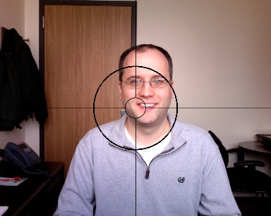

Figure 7-7. Example of painting crosshairs on an image

We can also manage layers independently of images. Because the scope marks are the same in each frame, we can draw them once and apply the layer to subsequent images. This reduces the amount of processing that must be done on each frame.

from SimpleCV import Camera, Color, Display, DrawingLayer

cam = Camera()

size = cam.getImage().size()

disp = Display(size)

center = (size[0] /2, size[1] / 2)

# Create a new layer and draw on it
scopelayer = DrawingLayer(size)

# This part works just like the previous example
scopelayer.circle(center, 50, Color.BLACK, width = 3)
scopelayer.circle(center, 200, Color.BLACK, width = 6)
scopelayer.line((center[0], center[1] - 50), (center[0], 0),
     Color.BLACK, width = 2)
scopelayer.line((center[0], center[1] + 50), (center[0], size[1]),
     Color.BLACK, width = 2)
scopelayer.line((center[0] - 50, center[1]), (0, center[1]),
     Color.BLACK, width = 2)
scopelayer.line((center[0] + 50, center[1]), (size[0], center[1]),
     Color.BLACK, width = 2)


while disp.isNotDone():
     img = cam.getImage()

     # Rather than a lot of drawing code, now we
     # can just add the layer to the image
     img.addDrawingLayer(scopelayer)

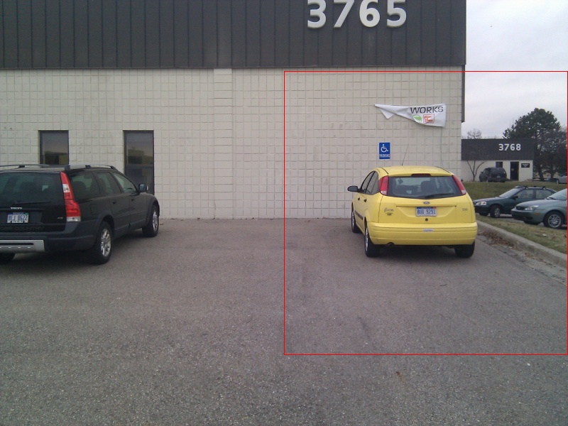
     img.save(disp)

When using markup on images, it’s often a good idea to use it to highlight regions of interest, as in this example which uses the parking photo first demonstrated in Chapter 4. To demonstrate to the application user the part of the image that will be cropped, we can draw a box around the relevant region:

from SimpleCV import Image, Color, DrawingLayer

car = Image('parking-car.png')

boxLayer = DrawingLayer((car.width, car.height))  

boxLayer.rectangle((400, 100), (400, 400), color=Color.RED)  

car.addDrawingLayer(boxLayer)  

car.show()

This block of code produces output as demonstrated in Figure 7-8.

Figure 7-8. Bounding box drawn around the yellow car

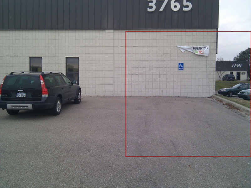
This layer can then be used to compare the crop region with the parking image without a car. This will help to compare the regions of interest between the two versions of the photos.

# This is a continuation of the previous example

nocar = Image('parking-no-car.png')

nocar.addDrawingLayer(boxLayer)

This works just like the previous example, except that now it shows the region of interest on the similar image without the illegally parked car. The resulting photo should look like Figure 7-9.

Figure 7-9. Box showing where the car is in the other picture

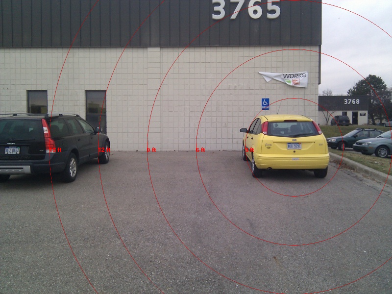
For a slight variation on the above example, drawing circles on the image could help to identify the distance between objects. For example, using the same example image as above, assume that 100 pixels is about 3 feet. How far away is the Volvo on the left from the illegal parking spot? One way to visually estimate the distance is to draw a series of concentric circles radiating out from the handicap parking space, as shown in Figure 7-9.

from SimpleCV import Image, Color, DrawingLayer

car = Image('parking-car.png')

parkingSpot = (600, 300)  

circleLayer = DrawingLayer((car.width, car.height))  

circleLayer.circle(parkingSpot, 100, color=Color.RED)  
circleLayer.circle(parkingSpot, 200, color=Color.RED)
circleLayer.circle(parkingSpot, 300, color=Color.RED)
circleLayer.circle(parkingSpot, 400, color=Color.RED)
circleLayer.circle(parkingSpot, 500, color=Color.RED)

car.addDrawingLayer(circleLayer)  

car.show()

The resulting image should look like the image in Figure 7-10. Based on the image, the car is four to five circles away from the center of the handicap spot. Because the radius increased by 100 pixels per circle, that translates into 400 to 500 pixels. Under the rough assumption that 100 pixels equals three feet, then the Volvo is currently around 15 feet away from the center of the illegal parking space. It is probably safe to assume that it is legally parked.

Figure 7-10. Circles approximating distance from the car

After all this drawing, it may be necessary to remove all the code and start over with a clean slate. To clear the image, use the clearLayers() function.

# This is a continuation of the previous example

car.clearLayers()

car.show()

print car.layers()

The car image is back to its original state before the circles were drawn. Visually, the circles no longer appear. When printing out a list of all the layers on the image, no layers appear. Note, however, that the original circleLayer object still exists. It can be placed back on the image with the addDrawingLayer() function.

This section did not cover all of the possible shapes, but it did present the standard approach. Several other frequently used options for drawing include:

Displaying text on the screen is fairly simple. In the previous example using circles to show distances, the example assumed that users knew that each circle was about three feet in radius. It would be better to mark those distances on the screen. Fortunately, drawing text on an image is just as easy as drawing shapes.

from SimpleCV import Image, Color, DrawingLayer

# This first part of the example is the same as before

car = Image('parking-car.png')

parkingSpot = (600, 300)

circleLayer = DrawingLayer((car.width, car.height))

circleLayer.circle(parkingSpot, 100, color=Color.RED)
circleLayer.circle(parkingSpot, 200, color=Color.RED)
circleLayer.circle(parkingSpot, 300, color=Color.RED)
circleLayer.circle(parkingSpot, 400, color=Color.RED)
circleLayer.circle(parkingSpot, 500, color=Color.RED)

car.addDrawingLayer(circleLayer)

# Begin new material for this example:

textLayer = DrawingLayer((car.width, car.height))  

textLayer.text("3 ft", (500, 300), color=Color.RED)  
textLayer.text("6 ft", (400, 300), color=Color.RED)
textLayer.text("9 ft", (300, 300), color=Color.RED)
textLayer.text("12 ft", (200, 300), color=Color.RED)
textLayer.text("15 ft", (100, 300), color=Color.RED)

car.addDrawingLayer(textLayer)

car.show()

Many of the components of this example should now be familiar based on previous examples. However, a couple of items are worth noting:

The resulting image should look like Figure 7-11.

Figure 7-11. Distance circles with labels

Although the red colored font is slightly easier to read than a simple black font, the labels are still a bit difficult to read. A larger, easier-to-read font would help. Changing the font is relatively simple. The first step is to get a list of fonts that are available on the system. The listFonts() function will do the trick:

# This is a continuation of the previous example

textLayer().listFonts()

This prints a list of all the fonts installed on the system. Actual results will vary from system to system. The name of the font is just the part between the single quotation marks. For example, u’arial' indicates that the arial font is installed. The u prefix in front of some entries merely indicates that the string was encoded in unicode. Because arial is a pretty common font on many systems, it will be used in the following examples.

To change the font, simply insert code such as indicated below before calling the text() function:

# Code you could add to the previous example

textLayer.selectFont('arial')  
textLayer.setFontSize(24)  

If used with the previous example, the output will look like the example in Figure 7-12.

Figure 7-12. Circles with larger, easier-to-read labels

Several other font configuration commands are also available:

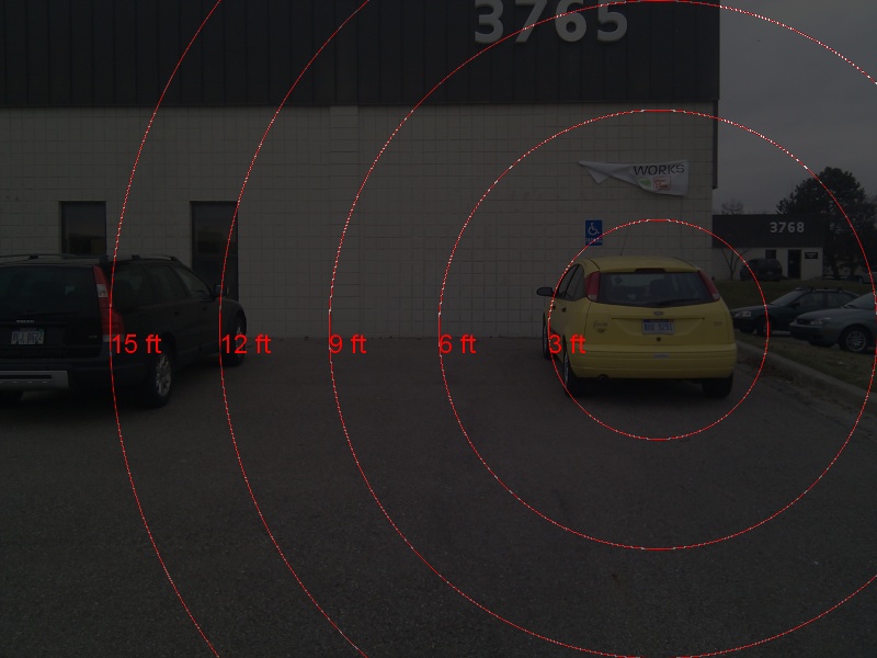
One final way to make it easier to see the drawn material is to control the layer’s transparency. By making it more opaque, it will mask the underlying material, making the drawn shapes and text stand out.

from SimpleCV import Image, Color, DrawingLayer

car = Image('parking-car.png')

parkingSpot = (600, 300)

circleLayer = DrawingLayer((car.width, car.height))

# This is the new part:
circleLayer.setLayerAlpha(175)

# The remaining sections is the same as before
circleLayer.circle(parkingSpot, 100, color=Color.RED)
circleLayer.circle(parkingSpot, 200, color=Color.RED)
circleLayer.circle(parkingSpot, 300, color=Color.RED)
circleLayer.circle(parkingSpot, 400, color=Color.RED)
circleLayer.circle(parkingSpot, 500, color=Color.RED)

car.addDrawingLayer(circleLayer)

textLayer = DrawingLayer((car.width, car.height))

textLayer.selectFont('arial')
textLayer.setFontSize(24)

textLayer.text("3 ft", (500, 300), color=Color.RED)
textLayer.text("6 ft", (400, 300), color=Color.RED)
textLayer.text("9 ft", (300, 300), color=Color.RED)
textLayer.text("12 ft", (200, 300), color=Color.RED)
textLayer.text("15 ft", (100, 300), color=Color.RED)

car.addDrawingLayer(textLayer)

car.show()

The one new line of code was using the setLayerAlpha function. This takes a single parameter of an alpha value between 0 and 255. An alpha of zero means that the background of the layer is transparent. If the alpha is 255, then the background is opaque. By setting it to a value of 175 in the example, the background is darkened but still visible, as is shown in Figure 7-13.

Figure 7-13. Partially transparent layer on top of the image

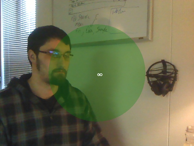
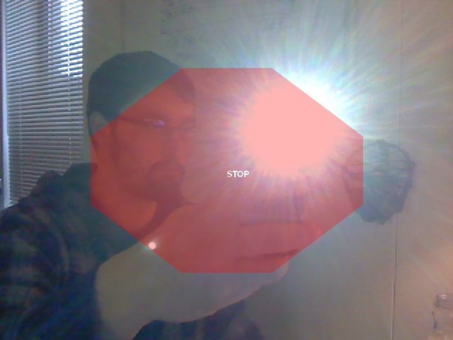
The two examples in this chapter demonstrate how to provide user feedback on the screen. The first example draws stop and go shapes on the screen in response to the amount of light captured on the camera. The second example expands on the crosshair code snippets above, integrating mouse events. Finally, the third example shows how to simulate a zoom effect in a window, controlled with the mouse wheel.

Making a Custom Display Object

This example is for a basic Walk or Don’t Walk type scenario, as shown in Figure 7-14 and Figure 7-15. It detects hypothetical vehicles approaching based on whether the light is present. If it detects light, it will show a message on the screen saying STOP.

Note

This example code is intended to demonstrate layers and drawing. It is not intended to be an actual public safety application.

from SimpleCV import Camera, Color, Display, DrawingLayer, np

cam = Camera()

img = cam.getImage()

display = Display()

width = img.width
height = img.height

screensize = width * height

# Used for automatically breaking up image
divisor = 5

# Color value to detect blob is a light
threshold = 150

# Create the layer to display a stop sign
def stoplayer():
     newlayer = DrawingLayer(img.size())  

     # The corner points for the stop sign's hexagon
     points = [(2 * width / divisor, height / divisor),
               (3 * width / divisor, height / divisor),
               (4 * width / divisor, 2 * height / divisor),
               (4 * width / divisor, 3 * height / divisor),
               (3 * width / divisor, 4 * height / divisor),
               (2 * width / divisor, 4 * height / divisor),
               (1 * width / divisor, 3 * height / divisor),
               (1 * width / divisor, 2 * height / divisor)
                         ]

     newlayer.polygon(points, filled=True, color=Color.RED)  

     newlayer.setLayerAlpha(75)  

     newlayer.text("STOP", (width / 2, height / 2), color=Color.WHITE)  

     return newlayer

# Create the layer to display a go sign
def golayer():
     newlayer = DrawingLayer(img.size())  

     newlayer.circle((width / 2, height / 2), width / 4, filled=True,
                    color=Color.GREEN)

     newlayer.setLayerAlpha(75)

     newlayer.text("GO", (width / 2, height / 2), color=Color.WHITE)

     return newlayer


while display.isNotDone():
     img = cam.getImage()

     # The minimum blob is at least 10% of screen
     min_blob_size = 0.10 * screensize

     # The maximum blob is at most 80% of screen
     max_blob_size = 0.80 * screensize

     # Get the largest blob on the screen
     blobs = img.findBlobs(minsize=min_blob_size, maxsize=max_blob_size)

     # By default, show the go layer
     layer = golayer()

     # If there is a light, then show the stop
     if blobs:
          # Get the average color of the blob
          avgcolor = np.mean(blobs[-1].meanColor())

          # This is triggered by a bright light
          if avgcolor >= threshold:
               layer = stoplayer()

     # Finally, add the drawing layer
     img.addDrawingLayer(layer)  

     img.save(display)

The stop sign will be a hexagon. The SimpleCV framework does not have a function specifically for drawing a hexagon; instead it needs a set of corner points that define the shape.

Use the drawPolygon() function and the list of corner points to construct the stop sign.

Set the layer’s alpha in order to partially gray out the background. Although the background is still visible, this helps draw attention to the stop sign.

Add text in the middle of the stop sign to say “Stop.”

The overall flow of this code is the same as in the previous steps, but it is slightly simpler because the sign is a circle instead of a hexagon.

Finally, add the layer. Depending on whether the light was shined at the camera, this will be either the stop sign or the go sign.

Keep in mind that lighting conditions and other environmental factors will affect how this application works. Play around with the threshold values to adjust the assurance. Although a train/traffic detector is a somewhat silly application, it demonstrates the basic principles behind detecting an object on the screen and then changing the screen output to alert the user—a very common activity in vision systems.

Figure 7-14. Example display when it is safe to walk

Figure 7-15. Example display when it is not safe to walk

from SimpleCV import Camera, Color, Display

cam = Camera()

size = cam.getImage().size()

disp = Display(size)

center = (size[0] /2, size[1] / 2)

while disp.isNotDone():
     img = cam.getImage()

     img = img.flipHorizontal()  

     if disp.mouseLeft:
          center = (disp.mouseX, disp.mouseY)  


     # The remainder of the example is similar to the
     # short version from earlier in the chapter

     # Inside circle
     img.dl().circle(center, 50, Color.BLACK, width = 3)
     # Outside circle
     img.dl().circle(center, 200, Color.BLACK, width = 6)

     # Radiating lines
     img.dl().line((center[0], center[1] - 50), (center[0], 0),
          Color.BLACK, width = 2)
     img.dl().line((center[0], center[1] + 50), (center[0], size[1]),
          Color.BLACK, width = 2)
     img.dl().line((center[0] - 50, center[1]), (0, center[1]),
          Color.BLACK, width = 2)
     img.dl().line((center[0] + 50, center[1]), (size[0], center[1]),
          Color.BLACK, width = 2)

     img.save(disp)

Image Zoom

The scroll wheel on a mouse is frequently used to zoom in or out on an object. Although most webcams do not have a zoom feature, this can be faked by scaling up (or down) an image, and then cropping to maintain the original image dimensions (see Figure 7-16). This example reviews how to interact with the display window, and it shows how to manage images when they are different sizes than the display window.

from SimpleCV import Camera, Display

cam = Camera()

disp = Display((cam.getProperty('width'), cam.getProperty('height')))

# How much to scale the image initially
scaleFactor = 2

while not disp.isDone():
     # Check for user input
     if disp.mouseWheelUp:  
          scaleFactor *= 1.1
     if disp.mouseWheelDown:
          scaleFactor /= 1.1

     # Adjust the image size
     img = cam.getImage().scale(scaleFactor)  

     # Fix the image so it still fits in the original display window
     if scaleFactor < 1:
          img = img.embiggen(disp.resolution)  
     if scaleFactor > 1:
          img = img.crop(img.width / 2, img.height / 2,
                    disp.resolution[0], disp.resolution[1], True)  

     img.save(disp)

Check if the mouse is scrolled up or down and scale the image accordingly. Each event increases or decreases the image size by 10%.

This step does the actual scaling. Note that at this step, the image is no longer the same size as the display window.

If the image is smaller than the display—as represented by a scale factor that is less than one—then it needs to be embiggened. Recall that embiggen() changes the canvas size of the image, but leaves the underlying image intact.

If the image is larger than the display, crop it. This example assumes that it should zoom into the middle. That means that the crop region is defined based on the center of the image. It is cropped to the same dimensions as the display so that it will fit.

Figure 7-16. Left: Camera zoomed out; Right: Camera zoomed in