
DSP application examples
It may be useful at this point to discuss in considerable detail some common DSP applications. Some of the contents of this chapter will be better appreciated after learning about digital filter design and implementations. However, these examples will help us recapture the broad picture of the usefulness of DSP in a variety of engineering areas.
The first application is on periodic signal generation using wave tables. Wave table generation techniques have become more popular with some of the new audio cards available for PCs. It is a very flexible way to generate periodic waveforms like sinusoidal waves. Wave table synthesis lies at the heart of many computer music application programs. This example also serves to illustrate the important concepts learnt in previous chapters on sampling.
The second application is in the area of communication systems. We shall describe the implementation of a certain wireless transmitter using DSP techniques. The specific advantages of this approach will be discussed. This example will illustrate the choice of sampling frequency or ADC resolution and the effects of these choices on the spectral characteristics of the generated signal.
The third application is in the area of speech synthesis. Speech synthesis is a very broad area that requires understanding of the characteristics of speech signals, phonetics, and at a higher level, linguistics. A simple way to model and synthesize speech signals by a model of the human vocal tract will be described. This application illustrates the filtering of some simple signals to create signals with certain desired spectral characteristics. The filtering required is in fact time varying.
We shall also describe some applications of DSP in image processing. Image (and video) processing is one of the major applications of DSP. Some photographic outlets offer instant photo enlargements and cropping, enhancement of old photographs, and other imaging services. None of these would be possible without the aid of DSP.
Finally, the application of active noise control will be discussed. Active noise control (ANC) is based on the simple physics of destructive interference of propagating acoustic waves. DSP systems are now powerful to enable real-time ANC systems to be developed with applications in air conditioning ducts, aircraft, cars and magnetic resonance imaging (MRI) systems.
5.1 Periodic signal generation using wave tables
Many DSP applications require the generation of periodic waveforms such as sinusoids, periodic square waves, sawtooth signals, etc. An example application is the generation of dual-tone multi-frequency (DTMF) signals for touch-tone telephone handsets.
Figure 5.1 shows the two frequency groups of a DTMF keypad.

When a key on the keypad is pressed, a signal, which is the sum of two audible sinusoidal tones, is generated. Each key on the keypad is uniquely defined by a frequency pair {fL, fH}, one from the low and one from the high frequency group. The digitally generated signal is mathematically given by
fs is the sampling frequency, and n is the integer time index.
5.1.1 Digital waveform generation using wave tables
One approach to generate such periodic waveforms is to design a digital filter with an impulse response h(n) corresponding to one period of the waveform, one wishes to generate. The periodicity is generated by exciting this digital filter with a train of impulses separated by the fundamental period of the waveform. This process is shown in Figure 5.2.

A more efficient approach is to pre-compute the samples of the waveform and store them in the system’s memory (RAM or ROM). The data are arranged as a circular buffer and accessed when needed. The period of the waveform can be controlled by either varying the speed of cycling around the table or by accessing a subset of the table at a fixed speed. This approach is called wave table synthesis, which is used very successfully in computer music. Many audio cards available for PCs now use wave table generators.
5.1.2 Sampling frequency
A sinusoidal signal does not necessarily remain periodic when sampled at a given frequency. In order that y(n) remains periodic in the time index n with a period of, say, D samples, it is necessary that one whole period of the sinusoid fit within the D samples. This requires that the sampling frequency is an integral multiple of the analog frequency f. That is,
Due to the periodicity, only the samples for one period of the signal need be calculated and stored. f is now the fundamental frequency of the wave table. A typical sampling frequency for DTMF generation is 8 kHz.
There are sinusoids of 8 different frequencies that need to be generated for DTMF signals. One way to do it is to have 8 wave tables. Since there are only a few entries per table, this approach is not impractical. Another way is to change the fundamental frequency using a single table. This is the approach that we shall examine in more detail.
5.1.3 Generating integer multiples of the fundamental frequency
The frequency f can be changed either by changing the sampling frequency fs or by changing the effective length D of the basic period. The first approach is not practical in our application since we need to deal with two different frequencies each time. Thus the second approach will be used.
The fundamental frequency generated from a wave table with D entries and a sampling frequency is given by
Replacing D by a smaller value, d will increase the frequency of the sinusoid. For instance, if d=D/2, the frequency is doubled. This also means that only every other entry in the wave table will be accessed for each period. So the new generated frequency will be
Given the desired frequency fd and a table length D, we will be using only c regularly spaced samples from the full wave table and c is given by
Now we have assumed that d and c are integers. This clearly restricts the choices of frequencies we can generate. We shall now consider how we can generate other frequencies where both d and c are real numbers.
5.1.4 Generating arbitrary frequencies
Any frequency f that we want to generate must be within the nyquist interval
This requires that c satisfies the condition
Negative values of c correspond to negative frequencies. This is useful for introducing 180° phase shifts in waveforms.
Since c is no longer an integer, some truncation or rounding will have to be done in order to get values from the wave table.
Alternatively, we can interpolate between sample values from the wave table for more accurate synthesis. Linear interpolation is usually sufficient. Let w(i) and w(j) be the i and j entries in the wave table and we need a sample with a real-valued index q which is between i and j. The linearly interpolated value is given by
This interpolation is shown in Figure 5.3.
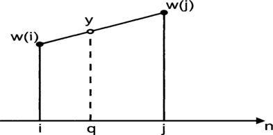
Interpolation naturally produces the most accurate results with rounding coming next. Truncation is the most inaccurate of the three methods. The inaccuracies become smaller as the length of the wave table D increases. In computer music applications, wave table sizes vary between 512 and 32 768.
5.1.5 DTMF example
Coming back to the generation of the DTMF frequencies. Assume that the sampling frequency is 8 kHz and the size of the wave table is 200. The fundamental frequency is therefore 400 Hz.
For the low frequency group, the values of c are given by

Similarly, the values of c for the high frequency groups are found to be 30.225, 33.4, 36.925 and 40.825.
5.2 Wireless transmitter implementation
A paging systems standard has been created in Europe in 1989 by the ETSI (European Telecommunications Standards Institute). It is called the ERMES (European radio message system). The main objective is to allow roaming throughout Europe and to guarantee receiver compatibility.
There is an older system called POCSAG, which transmits at 512 or 1200 bits per second. With new service needs foreseen in the most populated areas of Europe, ERMES was designed to transmit at 6250 bits per second. The modulation format that has been chosen is called 4-PAM/FM modulation. Since each symbol is encoded by two bits, the actual symbol rate is 3125 symbols (bauds) per second.
It is desirable to design a transmitter that can transmit using the older POCSAG system and the newer ERMES system. Such a flexible system will have the benefit of reduced system design cost. One way to achieve this flexibility is to implement it using DSP techniques.
Since radio spectrum is scarce, specifications for radio transmitters are very tight. The transmitters designed should be very precise and stable. Again, this is one of the major advantages of digital techniques and this points to DSP implementation.
5.2.1 Specifications
All the specifications of the modulation method can be found in
• ‘European radio message system – part 4: air interface specification’, ETSI DE/PS 2 01-4, version 0.2.1, November 1990.
• ‘European radio message system – part 6: base station conformance specification’, ETSI DE/PS 2 01-4, version 0.2.1, November 1990.
The modulated signal generation process is illustrated in block diagram form in Figure 5.4.
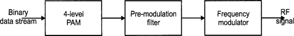
Using this technique, the communication of two data bits is achieved by the transmission of one of four signaling frequencies. The modulated signal is required to have a continuous phase (no sudden jumps in phase). This and the pre-modulation pulse shaping (or filtering) of the data stream constrain the transmitted radio frequency (RF) spectrum. The four signal frequencies are as shown below.
| Nominal frequency | Symbol |
| f0 + 4687.5 Hz | 10 |
| f0 + 1562.5 Hz | 11 |
| f0 − 1562.5 Hz | 01 |
| f0 − 4687.5 Hz | 00 |
Here f0 is the intended operating frequency. In a data stream, the most significant bit shall be transmitted first. The transmission rates are
The binary signal is filtered by the pre-modulation filter to create a smooth signal rather than one with sudden jumps in levels. The specifications for this filter are shown in Figure 5.5.
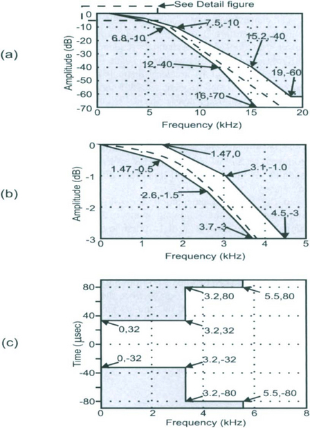
The specifications are given in terms of frequency characteristics with upper and lower limits. Apart from the amplitude spectrum, the phase spectrum is also specified as group delay characteristics. Group delay is defined as the negative rate of change of phase. So a constant group delay implies a linear phase function. In most cases for data transmission, this is the ideal. These specifications are derived from a 10th order low-pass Bessel filter with a 3 dB bandwidth of 3.9 kHz.
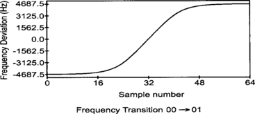
The rise or fall time for the frequency transition between two successive symbols shall be 88 microseconds with a tolerance of 2 microseconds.
The RF spectrum of the output of the transmitter shall conform to the mask shown in Figure 5.6.

The center frequency of the transmissions shall not exceed 15 Hz either way from the intended operating frequency (f0). The intended operating frequency may be forced to differ from the nominal channel frequency by up to 185 Hz (frequency offset). The difference between any two adjacent symbol frequencies shall be 3125 ± 15 Hz.
These specifications are very difficult to meet using conventional analog circuitry, especially the center frequency stability and the accuracy of the difference between two adjacent symbol frequencies.
5.2.2 DSP implementation
A classical way to generate a signal of this kind is to use an analog pre-modulation filter followed by an FM modulator. However, this approach presents problems regarding the stability of the parameters. It is very difficult to achieve a precision of 0.1% in the frequency deviation.
In the DSP implementation, the 4-PAM coder and the pre-modulation filter are implemented in the following manner. Since we have four possible symbols in the alphabet, there are a total of 16 possible transitions between symbols. These transitions are being smoothed by the filtering performed by the pre-modulation filter. All these 16 transitions and their corresponding results after filtering can be pre-calculated and stored in a ROM. In this way, the samples of the filtered signal are a function of the current and last symbol and can be looked up from the ROM.
In Figure 5.7, the transition between the symbol 00 and the symbol 10 is shown. The stored transition consists of 64 samples per symbol, 16 bits per sample.
The FM modulator block diagram is shown in Figure 5.8. The frequency samples obtained from the previous process are passed to an integrator, which is simply an accumulator of all past values.

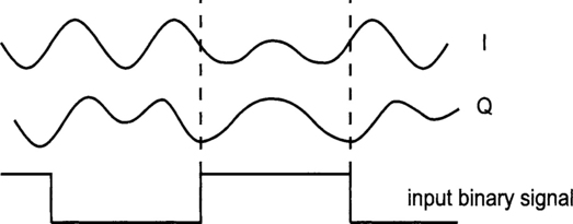
This generates the phase samples corresponding to the intended frequencies. The output from the integrator becomes the arguments of the sine and cosine tables. The cosine table gives the in-phase (I) component of the modulated signal and the sine table gives the quadrature (Q) component. The tables are quantized with 8-bit resolution. These samples are converted to analog signals using two DACs and a quadrature modulator, which can be obtained commercially as a chip, is used to generate the RF signal.
The specification allows frequency offsets that can be introduced intentionally. A very precise offset can be introduced by adding or subtracting a certain constant from the filter output samples.
POCSAG can also be implemented using the same scheme by including a different transition table corresponding to the POCSAG specification. In this way, the transmitter can switch between the two systems by simply getting its samples from a different table.
The symbol rate is low enough to allow us to choose the very high sampling rate of 64 samples per symbol. This high oversampling rate implies that very simple anti-aliasing filters can be used after the DAC. High sampling rate also reduces the time uncertainty of the transitions.
Figure 5.9 shows the analog I and Q signals generated with input symbols (10, 00, 10, 00).
5.2.3 Other advantages
There are some other advantages in using the DSP approach that may not be obvious initially. Two major ones are briefly discussed below:
• Quadrature modulator compensation
The quadrature modulator can process the I and Q signals to produce the RF output is an integrated circuit that consists of analog circuitry. Hence there are potential frequency offsets, and imbalance between the two channels. The result of these defects is generally a spread in the frequency spectrum. Since there are tight specifications on the allowable out-of-band power (at least 72 dB for ERMES), this spread in the spectrum may mean that these specifications are violated. If these imperfections can be modeled and the parameters of the model can be measured on-line or off-line, then compensation can be applied to the discrete-time signal before modulation so that the resulting modulated signal is near perfect.
• Power amplifier linearization
The most efficient power amplifiers have non-linear transfer characteristics. If the modulation format depends on the amplitude of the signal, then this non-linearity introduced by the power amplifier will severely distort the original signal. This is the reason why constant envelope type of modulations such as FM, is used in radio systems.
On the other hand, the most efficient modulation schemes do not produce constant envelope signals. Hence they require linear amplifiers which are much less efficient. By using DSP implementations, we can pre-compensate for the amplifier non-linearity by pre-distorting the discrete-time signal. In this way, the most efficient modulation schemes can be used with the most efficient power amplifiers. This is obviously not possible with analog implementations.
5.3 Speech synthesis
Digital speech processing has been one of the most important areas of DSP. It is the application of digital speech and image (including video) processing that leads to the explosion of multimedia communication that we are experiencing at the moment.
5.3.1 Speech production mechanism
Speech signals consist of a sequence of sounds. These sounds and the transition between them carry the information that needs to be conveyed. These sound sequences obey certain rules. Linguistics is the study of such rules for a certain language. The study of the classification of the basic sounds is in the realm of phonetics.
In order to come up with a model of speech production, we need to have an understanding of the human vocal system. It consists of two main parts: the vocal cords (or glottis), and the vocal tract. The vocal tract in turn consists of three main parts:
• The pharynx – connection from the esophagus to the mouth.
• The oral cavity – the mouth.
• The nasal tract – begins at the velum and ends at the nostrils.
The source of energy comes from the air pressure exerted by the lungs, bronchi and trachea. Speech is produced when an acoustic wave is radiated from this vocal system when air is expelled from the lungs and the air flow is perturbed by constrictions somewhere in the vocal tract. When the velum is lowered, the nasal tract is acoustically coupled to the vocal tract to produce nasal sounds.
5.3.2 Classification of sounds
The basic units of speech sounds in the English language are called phonemes. There are two main types of phonemes: vowels and consonants. More detailed classifications are also available. But for our discussions, we shall assume only these two types of sounds.
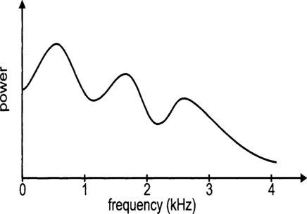
Vowels are produced when the vocal tract is excited by pulses of air caused by the vibration of the vocal cords. The vibration is periodic in nature and the period is the pitch of that sound. The shape of the vocal tract determines the resonant frequencies of the tract, called formants. For vowels, there are typically three formants between the frequencies 200 Hz and 3 kHz. The exact frequencies of the formants vary from person to person. Figure 5.10 shows a typical frequency spectrum of a vowel.
In the production of consonants, the vocal cord is totally relaxed in general, although there are exceptions. In this way, air flows into the vocal tract without the periodic excitation generated by the vocal cord. Consonants can be broadly classified into:
Nasals are produced when the vocal tract is totally constricted at some point along the oral cavity. The velum is lowered and the air flows through the nasal tract, radiating through the nostrils.
Fricatives are produced when the steady air flow becomes turbulent in the region of a constriction in the vocal tract.
Stops are transient sounds produced by building up pressure behind a total constriction somewhere in the oral tract, and suddenly releasing the pressure.
5.3.3 Speech production model
In order to synthesize speech sounds artificially; we need a model of the speech production system described above. We have looked at one briefly in Chapter 1. Figure 5.11 shows a more detailed model.

The glottal pulse model, the vocal tract model, and the radiation model are linear discrete-time systems. They are therefore essentially discrete-time filters. In order to synthesize speech, the voiced/unvoiced switch will switch to the source for the sound at that particular time. The vocal tract parameters will also need to vary with time.
One of the most successful glottal pulse models is the Rosenberg model. Its impulse response is given by
The vocal tract model is usually a linear predictive model. It is so called because the current speech sample is generated from a number of past samples plus the current
excitation. This can be described in equation form as
Here ak is the coefficient for the model and it changes from one phoneme to another, and u(n) is the input sample to the vocal tract model. The prediction order, p, is typically 10 to 12.
In most cases, the radiation model is ignored.
In the practical sessions, there will be an opportunity to experiment with the model.
5.4 Image enhancement
In this course, we only deal with the processing of one-dimensional signals and images are inherently two-dimensional. However, image processing is a very important DSP application area. We shall consider briefly the application of DSP techniques to the enhancement of images. This will give us some insights into what this area is about. Some operations are also non-linear as opposed to linear operations we have discussed so far.
Image enhancement is the processing of images to improve their appearance. There are a variety of methods, which are suitable for different objectives. Some objectives are to improve the image quality and visual appearance to a human viewer. Other ones include the sharpening of an image to aid in the automatic machine recognition of objects. But the overall objective is to make the processed image better in some sense than the unprocessed one.
We shall consider two types of enhancement: contrast and dynamic range enhancement, and noise reduction. For simplicity, we shall only use gray-scale images.
5.4.1 Contrast enhancement
A simple way to improve the contrast or the dynamic range of image pixel intensities is by a technique called gray-scale modification. It applies a transformation T to the original image to produce the enhanced image. This transformation is often represented by a table.
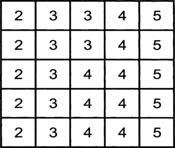
Consider an image of 5×5 pixels represented by 3 bits. There are a total of eight levels with 0 being the darkest to 7 being the brightest. The pixel values are shown in Figure 5.12. We can see that the pixel values are between 2 and 5. So only 4 out of 7 possible levels are used. Making use of the full range of values can produce a better contrast.
The problem is how we can find a suitable transformation that will do a good job. Computing the histogram of the image and studying its characteristics can identify a suitable transformation. The histogram is just a tabulation or a graph of the number of pixels that have specific intensities. The histogram of Figure 5.12 is shown in Figure 5.13.
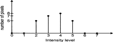
Figure 5.13 Histogram of the image in Figure 5.12
This histogram showed us that the dynamic range is not well utilized as discussed above. A transformation that will improve the contrast is shown in Figure 5.14 and the resulting output image after the transformation is in Figure 5.15.
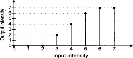
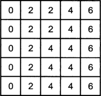
Figure 5.15 Image of Figure 5.12 after contrast enhancement transformation
The transformation can be obtained automatically by defining a desired histogram. In most cases, the desired histogram is usually a uniform distribution of gray level values within the image. This will make the number of pixels at any one gray level about the same as another. The transformation T must be monotonically non-decreasing like the one in Figure 5.14. It is given by
where N is the total number of pixels in the image, ni is the number of pixels at gray level i, and M is the total number of gray levels possible.
This simple procedure often produces significant improvements in image quality or intelligibility to the viewer.
5.4.2 Noise reduction
There are two main types of noise in images. One is the uniform random noise similar to those for one-dimensional images. Another type one is known as impulse noise or salt-and-pepper noise. They appear as isolated bright or dark pixels in the image. They can occur due to random bit error during transmission.
The energy of a typical image is primarily in the low frequency region. Therefore, (two-dimensional) low-pass filtering will be quite effective in removing a substantial amount of uniform random noise. This is done at the expense of removing some details of the image. It should be noted that edges that exist in the image produce high frequency components. If these components are removed or reduced in energy, then the edges will become fuzzier.
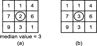
Median filters are very effective in removing impulse noise while preserving edges. They are non-linear filters however, and therefore the process cannot be reversed. In median filtering, a window or mask slides along the image. This window defines a local area around the pixel being processed. The median intensity value of the pixels within that window becomes the new intensity value of the pixel being processed.
Figure 5.16(a) shows a 3×3 window. The pixel being processed in the middle of this window. The numbers within the window are the intensity levels of the pixels in that window. Figure 5.16(b) indicates the processed output. Note that the intensity of the pixel in the middle is now replaced by the median value.
An important parameter in median filtering is the size of the window. Different results can often be obtained by using different window sizes. The choice also depends on the characteristics of the image and the noise. As a rule of thumb, images with lots of variations require the use of smaller windows while larger windows can be applied to images that have more uniform intensity areas.
5.5 Active noise control
Active noise control (ANC) is based on the simple physics of destructive interference of propagating acoustic waves. The concept that acoustic wave interference can be controlled to produce zones of quietness has been known since sounds waves were first modeled by linear equations. In fact, a US patent was granted in the 1930s for an analog ANC system. DSP devices are now powerful enough to allow us to design and implement digital ANC systems that operate in real-time.
Figure 5.17 illustrates the subsystems involved in a single channel digital ANC system. The secondary loudspeaker produces an acoustic signal, which on arrival at the error microphone, is a 180° phase-shifted version of the original signal d(k). If

then the resulting error signal e(k) obtained through the error microphone is zero and a zone of quietness is setup around the error microphone. Owing to the complex nature of even the simplest acoustic environment, in practice zero error is unlikely to be achieved.
Figure 5.18 shows a system block diagram, which models the system in Figure 5.17. Here He(z) models the acoustic path from the loudspeaker to the error microphone, and Hr(z) models that from the loudspeaker to the reference microphone. The reference microphone provides the noise controller with an input signal whose spectral content is similar to that of d(k). The reference microphone signal is linearly filtered to produce an appropriate loudspeaker output y(k). The active noise controller is modeled by W(z).
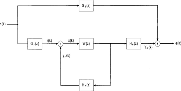
If we want e(k) = 0, without going into the details, the transfer function of the ANC filter is required to be as follows:
This is an analytical solution to the problem provided we have full knowledge of the characteristics of the acoustic paths. This is generally not the case. Furthermore, acoustic path characteristics may change with time since they are affected by events such as movements of objects within the location concerned. Most practical ANC systems therefore use adaptive filtering techniques, which allows the system to adaptively model the acoustic paths. It also has the advantage that the adaptation algorithm can devote its efforts to solve for Wreq(z) only for those frequencies, which are actually contained in the noise signal. In this way, more efficient use of the filter coefficients can be obtained.
It should be noted that many adaptation algorithms require prior knowledge of the acoustic path He(z) in order to solve for Wreq(z). Fortunately, the impulse response is usually well defined and easily measurable.
The inherent filter inside the active noise controller can either be an FIR or an IIR filter. As we shall see in the next two chapters, there are advantages and disadvantages for each type of filter in this application. FIR filters are stable and the equations for solving for the filter coefficients are easier to handle compared with IIR filters. But the order of FIR filter required is much higher compared to an IIR filter with similar spectral characteristics.
The filter weights are usually adapted or updated using a least-mean-squared (LMS) type of algorithm. This type of algorithm basically attempted to minimize the mean of the error signal squared, i.e. e2(k). At each iteration k, the filter coefficient w(k) are updated using the currently available information. The simplest updating formula is given below:
In this formula, the parameter μ affects how fast the coefficients are changing. μ is typically much less than 1 to ensure stability of the algorithm.
Block diagram of an LMS adaptive algorithm for an IIR filter system is shown in Figure 5.19. A(z) and B(z) are the transfer functions related to filter coefficients.

The order of the filter used is dependent on the complexity of the acoustic path He(z) that is reflected by the impulse response of this path. Filter orders between 100 and 200 are not uncommon. Naturally, the filter order is also dependent on the sampling frequency since it affects the total delay that the filter can model. For instance, a sampling frequency of 2 kHz has a sampling period of 5 ms, so a filter order of 100 can model an acoustic path delay of 500 ms or half a second.
To create a larger or multiple zones of quietness, we can use a multi-channel noise controller similar to the one illustrated in Figure 5.20.

To get a feel of the values of the parameters used, let’s consider a MRI system. MRI scanners produce very high levels of low frequency acoustic noise, which can make the scanning procedure very traumatic and also interfere with patient-operation communication. A two-channel ANC system could be used with a 120th order FIR filter operating at a sampling frequency of 2 kHz. Frequencies below 350 Hz are reduced by around 10-20 dB but those frequencies above 350 Hz are not reduced so that voice communication between patient and operator is not affected.
5.6 To probe further
We can only touch on a few applications in several areas that may be of interest to our readers. As indicated in chapter 1, DSP application areas are very broad. A good source of review articles can be found in ‘IEEE signal processing magazine’
Other popular electronics magazines also feature practical projects using DSP techniques.