In previous chapters I introduced several of the pillars of Haskell programming: the pure functional paradigm and the strongly typed nature of the language, which nevertheless allows powerful type constructs such as parametric polymorphism and type classes. This chapter will be devoted to understanding the unique evaluation model of Haskell, based on laziness , and the consequences of that choice.
In short, lazy evaluation means that only the necessary parts of an expression are computed, and this is done at the last possible moment. For example, if you have an expression such as head [2+3, 5*7], the multiplication is never performed at runtime because that value is irrelevant for the result of the expression. head uses only the first element in the list. As you may know, this way of performing evaluation is quite different from other programming languages. That opens the door to some interesting new idioms, such as working with infinite and cycling structures without caring about their special nature.
However, as a developer, you also need to be conscious of the trade-offs this model has, especially in the area of memory usage and performance. You will see the most typical problems that arise because of the laziness in Haskell code and learn about Haskell’s strictness to overcome them. Strictness annotations are available in pattern matching and in data declarations. The time and memory profiler that comes bundled with GHC will be an incredible tool to spot these problems; in this chapter you will look at its basic usage.
An Infinite Number of Time Machines
First you are going to see how Haskell can cope with infinite and cyclic structures without imposing any burden on the developer. In this section, you will look at the declaration and usage of these kinds of values in an intuitive way. The next section will discuss how Haskell is able to represent this information so that the code works.
Somehow, Haskell knows how to treat an infinite list, given that you observe only a finite part of it during runtime. On the other hand, the evaluation of an expression such as length timelyIncMachines involves traversing the entire list, so it doesn’t end.
Note
The notation [e ..] does not necessarily imply that an infinite list is created but rather that the list will hold all the elements larger than e. For example, [False ..] is equivalent to writing [False, True] because the ordering in Bool is False < True and there are no more elements in that type.
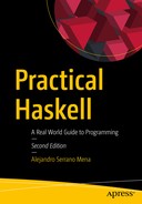
Properties of the list of Fibonacci numbers, graphically
In Exercise 5-1 you will see how infinite lists can even give you a glimpse into history.
Exercise 5-1: The Sieve of Eratosthenes
Start with a list of all the numbers from 2 on.
Take the first number, in this case 2, and drop from the list of numbers all its multiples, that is, all numbers n such that the remainder of n and 2 is 0.
Now take the next number (in this case it will be 3) in the filtered list and repeat the operation: filter out all the multiples of that number.
Repeat the previous step with the first number left in the previous one.
Implement the sieve of Eratosthenes using the techniques outlined in this section. The solution should take the form of a declaration primes :: [Integer], which contains all the prime numbers.
Lazy Evaluation Model
At this point, you should be convinced that Haskell can indeed work with infinite values (or, at least, with infinite lists). However, it may seem a bit like black magic. Of course, this is not the case: the ability to work in this way is the result of the strategy that Haskell follows for evaluating expressions, which departs greatly from other programming languages. In this section, I will introduce this lazy strategy and point out some of the most common problems with it.
Understanding Evaluation in Haskell
In contrast, Haskell tries to evaluate expressions as late as possible. In this example, it won’t initially evaluate the expressions that make the elements in the list. When it finds a call to head, it obtains the first element, which will still be an unevaluated expression, 3+2. Since you want to print the result of this expression on the screen, it will continue only by computing the addition, until it arrives at the same final value, that is, 5. This kind of evaluation is known as nonstrict or lazy.
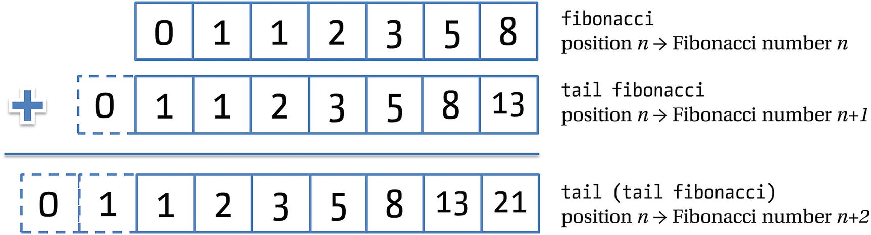
I have been intuitively using the idea of “evaluating as late as possible.” But that approach is not directly applicable to the example of the infinite list because for getting the head you have to enter the body of timeMachinesFrom, which would then give rise to a loop. The extra bit of information you need to know is that, by default, Haskell evaluates an expression only until a constructor is found. The rest of the value will be left unevaluated. Its spot will be occupied by a placeholder indicating how that specific field can be computed. This placeholder is called a thunk.
Evaluation of head timelyIncMachines

(head allNumbers, head (tail allNumbers), tail allNumbers)
Exercise 5-2: Evaluating Fibonacci
Write down the evaluation steps of the expression fibonacci !! 3, where fibonacci is the infinite list of the Fibonacci numbers, as defined previously in this chapter.
This would be impossible in a language that allows printing while computing a value. Let’s assume than during its evaluation allNumbers outputs "Natural numbers rule!". If you share the same value for allNumbers, the string would be printed only once. But in many languages, including C and Java, what you would expect is to show it three times, one per reference to allNumbers. You have seen that side effects make it impossible to apply these sharing optimizations, which are key to good performance in Haskell programs.
Even though allNumbersFrom 1 will call allNumbersFrom 2, the evaluation of allNumbersFrom 2 in allNumbersFrom 1 and in the previous expression will not be shared.
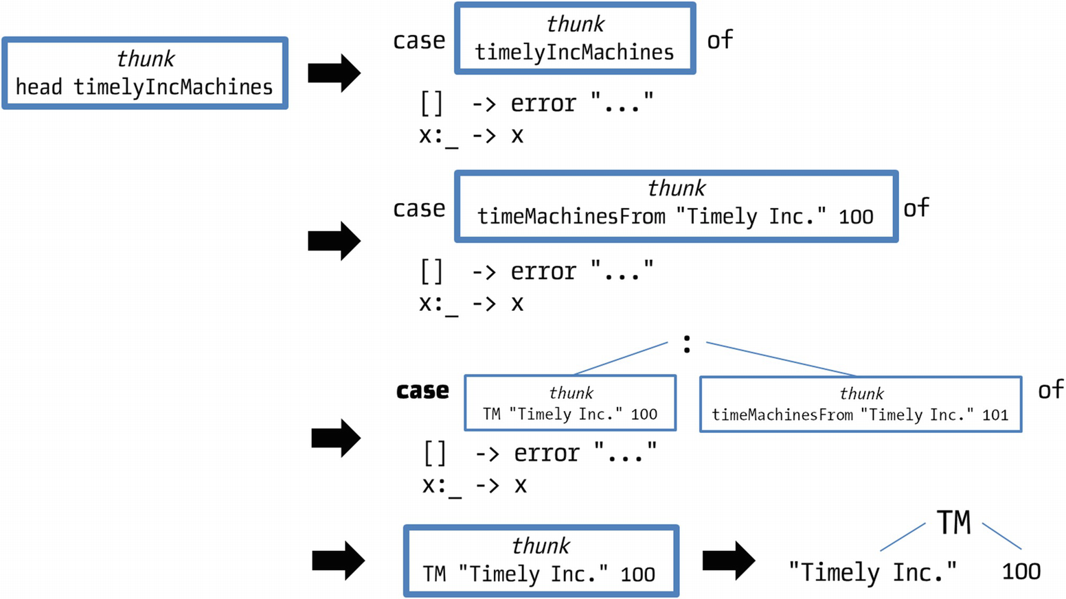
Evaluation of repeat e
Evaluation Strategies
In this section you saw two examples of evaluation strategies: ways in which the computation proceeds and the order in which parts of the expressions are evaluated. In addition to those two, more strategies have been developed.
What I have called strict evaluation is also known as call by value. Sometimes, especially in object-oriented languages, this is changed to call by reference, where you don’t receive values as arguments but boxes holding those values.
Lazy evaluation is sometimes referred to as call by need, which is a special case of the more general strategy of call by name, in which function arguments are not evaluated before the body of the function but are substituted directly. The difference is that, in general, call by name may evaluate the same expression more than once, whereas call by need uses thunks to do it only once.
Problems with Laziness
Laziness is often a blessing, but sometimes it can also be a curse. As usual in computer science, there’s a trade-off in lazy evaluation. In this case, delaying the evaluation until needed may result in less computation and also allow some programming idioms unavailable in other languages. On the other hand, it may create many thunks, causing the memory to become quite full so that the operating system starts to paginate, which makes the program slower. Let’s look at this problem with the help of your old friends, the folds.
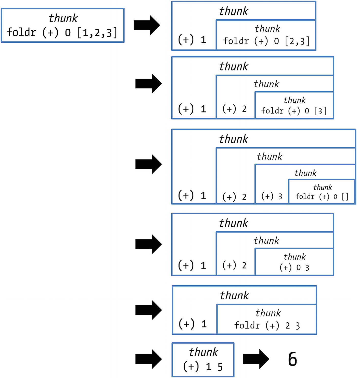
Evaluation of foldr (+) 0 [1,2,3]
Note
At first sight, the culprit could also be the big length of the list. However, if you perform some other computation over it that doesn’t create thunks in between, such as length [1 .. 1000000000], you can see that the system responds correctly (the actual speed will depend on the capacity of your computer to hold big integers).
But here you face a similar situation: (+) has at each step all of its arguments, but since you do not request the result until the end of the list, many thunks have to be created.
When executing sumForce [1 .. 1000000000], the interpreter may take a lot of time, but no memory problem will arise, and eventually an answer will be given. The idiom x `seq` f x is so common that there is a special operator, $! (strict application), to perform this task. So, you can rewrite the bold expression in the previous piece of code as sumForce' ys $! (z+y).
Note
Once again, you see a familiar foldlike pattern in the previous code. Prelude includes a foldl' function that forces the accumulated value before passing it into the next step. To avoid a memory leak you could have written the previous example as foldl' (+) 0 [1 .. 1000000000].
Once again, I stress that Haskell evaluates something only until a constructor is found. The fields are left as thunks until some further computation needs the information enclosed by them. This is true also for seq. If you want to be sure that some part of a larger value is evaluated before continuing, you should explicitly get that value and force it (you will see by the end of the chapter that if you don’t want any thunk inside a value, you can use deep strict evaluation with deepseq ). This is enough for this case because the first constructor that will be encountered will be the integer value coming from the addition.
Now that you know about forcing evaluation, you should resist the temptation to use it everywhere you think a memory problem could be found. Forcing expressions destroys the lazy nature of the language and may also lead to cases where a previously terminating expression no longer is. Think of the case of taking the head of an infinite list. If you make Haskell force the entire list, it will never reach the end, thus entering into an infinite computation chain. If you suspect a memory leak, you should first use profiling to find the correct spot and then think carefully whether using seq will not hurt the applicability of your functions to the kind of arguments that are expected.
Pattern Matching and Laziness
As you can see, this interplay of delays using thunks and forcing their evaluation is important. For that reason, you should have a clear idea of when computation takes place. In addition to explicit seq or ($!), another place where the compiler or interpreter needs to evaluate thunks is on pattern matching; it needs to evaluate up to the point that it knows which of the corresponding branches has to be taken.
Interesting enough, and because of this evaluation forcing in pattern matching, Haskell also includes a way to delay evaluation in matching phases. The way to do it is to use an irrefutable pattern. Matching upon it never fails, but it’s destructured only when some of its constituent parts are needed. One use case for irrefutable patterns involves a function that always returns a value given the same input. For example, you are finding an element in a list, and you have made sure that the element you are searching for already exists, so find will always return the same result. In that case, you can delay the computation of find a bit and just evaluate it when you need the constituent value.
Note
Irrefutable patterns are rarely used, but in some cases they are the key to code that performs well. You shouldn’t worry too much about understanding all the cases where they may be applicable, but knowing of their existence may become handy, especially if reading the source of some built-in function.
Strict Functions
It won’t be long until you read in the documentation of some package that a function is strict on one or several of its arguments. At a high level, this means the argument will have to be evaluated if it is still in thunk form, so you should take care of providing in that place an expression that won’t lead to nontermination.
Formally, in Haskell there is a canonical value called undefined that represents all those computations that don’t end. Because undefined never returns, it can be typed as you want, so you can have undefined :: a. By the way, this typing makes undefined a perfect placeholder in the place of code you haven’t yet written, such as when you want to check that your current code passes type checking.
A function f is then called strict on its argument if f undefined = undefined; that is, if given a nonterminating argument, the function itself does not terminate. One example of a strict function is head. But a function defined as g x = 1 isn’t, because, given any argument, it returns 1.
Intuitively, the notion of being strict on something means that it doesn’t inspect that something. The way a function is strict may be subtler than in the previous examples. For example, head undefined is undefined, but head (1 : undefined) isn’t.
Profiling with GHC
The GHC compiler can be used to generate statistics about runs of your program to get more insight on where computation effort is spent. In this section you will focus on two kinds of profiling: time profiling , which gets information about the amount of time spent in each of the functions in the system, and memory profiling, which allows you to look at the values holding the larger amount of memory. The profiling output in GHC assigns time or memory to the so-called cost centers, and the information and summaries are always related to them. By default, cost centers are assigned to functions, but more can be added using annotations.
To use profiling, you can no longer build the code as a library. You need to build a full executable that could be run from the command line. So, let’s first look briefly at the modifications you need to do in the Cabal file to include an executable.
Each Haskell project may include several executables, identified by a name, and with a reference to the file that includes the entry point of the application as a function main of type IO (). For now, it’s only important to know that IO allows you to perform side effects such as printing onto the screen; you will take a closer look at this type in Chapter 9. Each of these executables is defined as a new block in the Cabal file. The name is specified after the executable keyword that heads the block, and the file containing the entry function is declared inside the main-is property. It’s important to note that the main-is property needs a reference to the file itself (including the extension), not a module name like other properties. The auxiliary modules are defined inside the other-modules property, and dependencies are specified in the build-depends property, as in library blocks.
The information is divided into three parts. The first part is a summary of the total time and memory used by the program. The second part shows the cost centers (in this case, functions) that contribute the most to that cost. In this case, it’s obvious that result takes most of the time and memory, and main uses a smaller part of it. The last part is a more detailed view that shows the information about time and allocation in a tree. In this case, a lot of internal functions dealing with file handles and encoding are shown, but in a larger application fewer of these will be shown because they will be buried in a larger call stack.
However, the most interesting part is heap profiling, which allows for the production of a graph stating the consumption of memory throughout the program. The most important ways to run heap profiling are breaking it down by cost centers, which is specified using the -h runtime option, and breaking it down by type, whose option is -hy. Other ways to group consumption, such as by module, by closure, and so on, are available but not used often. If you run the previous program with any of those options, a new file is produced, called profiling-example.hp. This file is raw information; to convert it to a graph, you have to use the hp2ps tool that comes bundled with the Haskell Platform. Running hp2ps -c profiling-example.hp will produce a (color) PostScript file that can then be viewed.
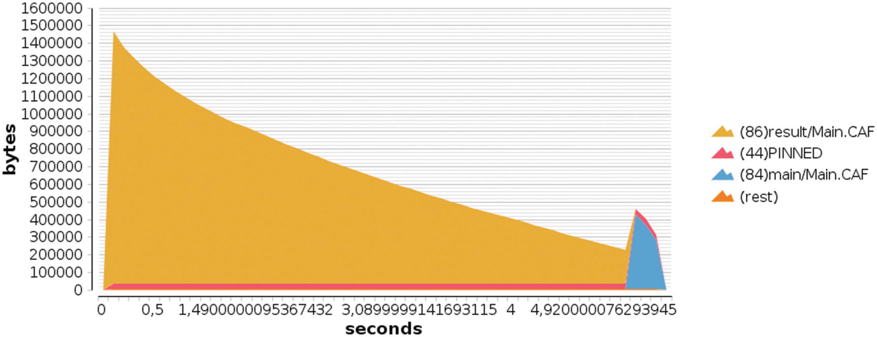
Graphical output of heap profiling by cost centers (run with -h)
You can see here that there is a big increase in memory usage in the first tenths of a second, shown in orange. This reflects the large creation of thunks I spoke about in the “Problems with Laziness” section. Then, the memory decreases as the thunks are evaluated. A second spike, shown at the extreme right edge of the graph, highlights the increase in memory when the resulting number has to be converted to a string.
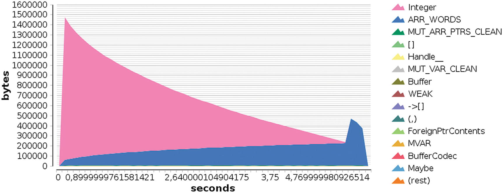
Graphical output of heap profiling by types (run with -hy)
As you can see, at the beginning most of the memory belongs to elements of type Integer, which corresponds to those thunks I talked about. As you go further in the execution, the ARR_WORDS type uses more memory. This encompasses the memory used by basic types such as evaluated integers (you see that it grows as the number gets larger) and strings.
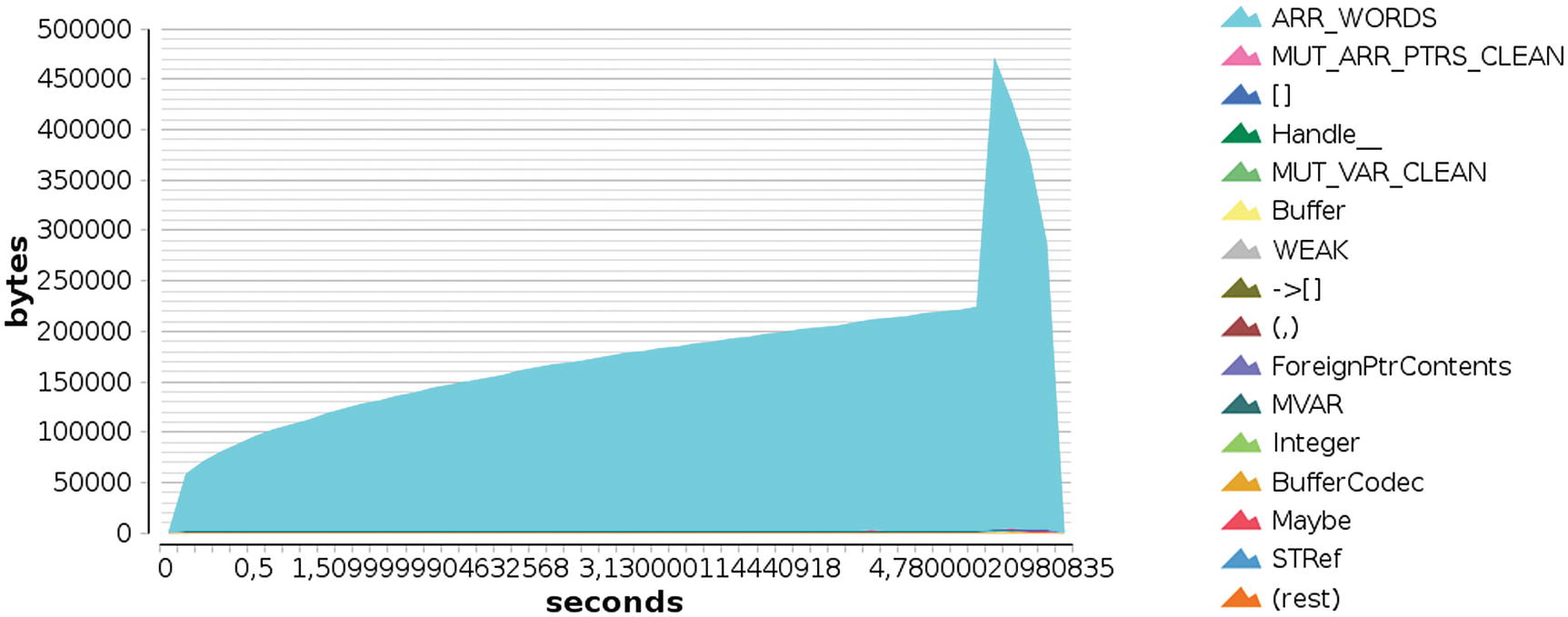
Graphical output of heap profiling by types, foldl' version
As you have seen, profiling is a great tool for spotting problems both in time and in memory because it allows focusing on those points that are really wasting those resources, instead of having to guess where the leak comes from. I suggest profiling some larger programs to get confident with the profiler and its output in order to be productive with the tool in the near future.
Strictness Annotations
This section gives more insight into GHC internals. You may safely skip this section in a first reading, but you should return to it later because you will greatly benefit from this information. This section will help you understand the memory and time used by your problem, and it gives you the tools to enhance your application in those aspects.
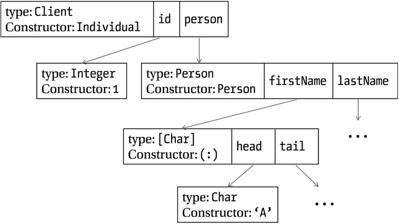
Representation of Individual 1 (Person "Andrea" "Blacksmith")
Remember that before being completely evaluated, expressions in Haskell are represented by thunks. Figure 5-9 shows the memory representation when an expression is completely evaluated. If some parts of it were still to be computed, the references will point to thunks containing the code to be executed.
This representation is flexible but suffers from some performance penalties. First, you may be creating thunks for values that you know will be used in the future or that may be needed to ensure good performance for that data type. For example, if you implement a new kind of list that stores its length, it doesn’t make much sense to not store the length directly and instead evaluate it lazily because at the moment you need to query it, a long chain of computations will happen and performance will suffer.
The memory representation of values also makes generous use of references to associate values with field positions. This means every time you want to access a field in a value, you need to traverse one reference. Once again, this is flexible and allows you to have potentially extensive structures in memory. However, it can be overkill for accessing small fields, such as integer ones, whose value could be directly encoded in the space that is taken by the reference (the size of a pointer in the target architecture). A field in that situation is said to be unpacked.
Note that not all fields can be unpacked; it depends on the type of field. Basic types, such as integers or characters, are eligible. Other data types can be used only if they consist of just one constructor and all their fields are also unpacked. This makes it possible to unpack a tuple of types that are unpackable themselves but forbids unpacking a list. Trying to unpack a String field will also produce a warning since it’s just a list of Char.
In many cases, you should consider whether for your particular application you prefer a lazier or a stricter implementation of your data structures. Laziness delays the moment of evaluation and allows you to compute only what is strictly needed for the program but has the trade-offs of larger memory consumption and more uncertainty over when the evaluation will take place.
Some packages, such as containers, provide both lazy and strict implementations of the data structures. For example, you have both implementations of maps living in different modules: Data.Map.Lazy and Data.Map.Strict. By default, the module Data.Map uses the lazy versions. The difference in this case, stated in the documentation, is that in the strict version both keys and values are forced before being saved in the map, whereas in the lazy version this is done only for keys.
Even Deeper
In some cases you need to evaluate an expression until no thunks are left. For that matter, the Haskell Platform provides the deepseq package , which in its module Control.DeepSeq provides the deepseq and ($!!) functions, similar to seq and ($!), respectively, but that also takes care of forcing the subexpressions, not stopping at the layer of constructors.
If you want your data types to support deep evaluation with deepseq, you have to make them instances of the NFData type class. Implementing them is quite easy; you just need to force all the fields and then return (). Here’s an example, in Client:
import Control.DeepSeq
instance NFData Client where
rnf (GovOrg i n) = i `deepseq` n `deepseq` ()
rnf (Company i n (Person f l) r) = i `deepseq` n `deepseq` f `deepseq` l
`deepseq` r `deepseq` ()
rnf (Individual i (Person f l)) = i `deepseq` f `deepseq` l `deepseq` ()
The same warnings for forcing with seq apply to deepseq, but they are even stronger because the latter forces even more evaluation to take place.
Summary
You saw how lazy evaluation allows you to work with seemingly infinite or cyclic structures, making for elegant patterns in the code.
I explained the lazy evaluation model, explaining the special role of thunks for delaying evaluation until a value is needed and at the same time increasing sharing of evaluated computations.
You looked at the shortcomings of lazy evaluation, the most important being increased memory consumption and uncertainty about the moment in which a thunk will become evaluated.
You learned how to annotate the code using seq, or strictness annotations in both pattern matching and data types, to work around these problems.
The GHC profiler is a powerful tool for detecting time and space leaks. I covered its basic usage and the interpretation of its results in this chapter.