Boosting

Just like random forest, GBM is an ensemble method: we’re going to be making more than one tree, then combining their outputs. Boosting is the central idea here. What is getting the “boost” is the importance of the harder-to-learn training data. Imagine a data set with just 10 rows (10 examples to learn from) and two numeric predictor columns (x1, x2), and we are trying to learn to distinguish between two possible values: circle or cross.

The very simplest decision tree we can make has just one node; I will represent it with a straight line in the following diagrams, which divides our training data into two. Unless we get lucky, chances are it has made some mistakes. Figure 6-1 shows the line it chose on its first try.

The truth table from our first decision tree looks like:

           Correct
       Circle  Cross
 Circle   3      1
 Cross    3      3

Figure 6-1. First try to partition the data

It scored 60%: six right, four wrong. It called one cross a circle, and there were three circles it thought were crosses. What we do now is train another very simple tree, but first we modify the training data to give the four rows it got wrong a higher weight. How much of a higher weight? That is where the “gradient” bit of GBM comes in (but we don’t need to understand it to use and tune GBMs).

In Figure 6-2 I’ve made the circles and crosses for the wrong items bigger, and our next tree pays more attention to them.

It helped, as it got three of those four right… But it got a different three items wrong, so it still scores 60%. So, for our third tree, we tell it those four are more important; the one it has got wrong twice in a row is the biggest of all. Figure 6-3 shows its third attempt.

If we stop training here, we end up with three weak models that scored 60%, 60%, and 80%, respectively. However, at least one of each of those three trees got every training row correct. You can see how they can work together to cover each other’s weaknesses, but hopefully you also got a glimpse of how easy it would be to overfit the data.

Figure 6-2. Second try to partition the data

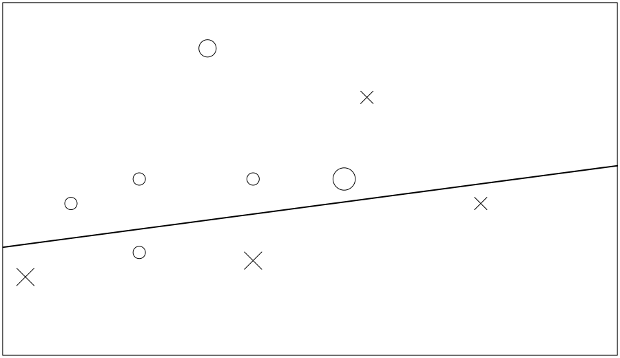
Figure 6-3. Final try to partition the data

The Good, the Bad, and… the Mysterious

GBM naturally focuses attention on the difficult rows in your training data, the ones that are hard to learn. That is good, but it can also be bad. If there is one outlier that each tree keeps getting wrong it is going to get boosted and boosted until it is bigger than the whole universe. If that outlier is real data (an unusual event, a black swan), then this is good, as it will know what to do when it sees one again. If it was bogus (a measuring error, a typo) it is going to distort your accuracy.

The H2O implementation of GBM works well across a cluster if your data is large. However, in my tests, there was not much speed-up from using a cluster on smaller data sets.

The mysterious? Well, unlike (simple) decision trees, which can be really good at explaining their thinking, it becomes a bit of a black box. You have all these dumb little trees, yet quality answers kind of emerge out of them.

Parameters

If you read Chapter 5, you will have seen most of these, but the relevant ones will be shown again here. learn_rate, learn_rate_annealing, and max_abs_leafnode_pred are GBM-specific. What random forest calls mtries, GBM calls col_sample_rate; see “Sampling, Generalizing” in Chapter 4—in fact, see the whole of that chapter for the other parameters you can use to control GBM.

For Python users, all of the following parameters are given to the model’s constructor, not to the train() function.

Just as with random forest, the two most important parameters are:

ntrees

How many trees to make.

max_depth

How deep each tree is allowed to grow. In other words, how complex each tree is allowed to be.

GBM trees are usually shallower than random forest ones, and that is reflected in the lower default of 5 for max_depth. ntrees defaults to 50 (same as random forest).

These two control the learning rate:

learn_rate

Learning rate (from 0.0 to 1.0). The default is 0.1. Lower takes longer and requires a higher ntrees, both of which will increase training time (and query time), but give a better model.

learn_rate_annealing

Scale the learning rate by this factor after each tree (e.g., 0.99 or 0.999). This defaults to 1.0, but allows you to have the learn_rate start high, then gradually get lower as trees are added.

The next two parameters control if splitting is done:

min_rows

How many training data rows are needed to make a leaf node. The default is 10; if you set it lower you may have more of a problem with overfitting.

min_split_improvement

This controls how much reduction in the inaccuracy, in the error, there has to be for a split to be worthwhile. The default is zero, meaning it is not used.

The next set of parameters control how the splitting is done:

histogram_type

What type of histogram to use for finding optimal split points. Can be one of “AUTO,” “UniformAdaptive,” “Random,” “QuantilesGlobal,” or “RoundRobin.” Can usually be left as AUTO, but worth trying in a grid if you are hunting for ideas.

nbins

For numerical columns, build a histogram of (at least) this many bins, then split at the best point. The default value is 20. Consider a lower value if cluster scaling is poor.

nbins_top_level

For numerical columns, build a histogram of (at most) this many bins at the root level, then decrease by factor of two per level. It defaults to 1024.

nbins_cats

For categorical columns, build a histogram of (at most) this many bins, then split at the best point. Higher values can lead to more overfitting, and also worse performance on a cluster. Like nbins_top_level, the default is 1024.

Finally, there is this one for when you are running on a cluster, but find it scaling poorly:

build_tree_one_node

Run on one node only. You will only be using the CPUs on that node; the rest of the cluster will be unused.

Regarding scaling, the communication overhead grows with the number of calculations to find the best column to split, and where to split it. So more columns in your data, higher value for nbins and nbins_cats, and a higher value for max_depth will all make it scale less well.

Building Energy Efficiency: Default GBM

This data set deals with the heating/cooling costs of various house designs (see “Data Set: Building Energy Efficiency”), and it is a regression problem. If you are following along, run either Example 3-1 or Example 3-2 (from Chapter 3), which sets up H2O, loads the data, and has defined train, test, x, and y. We are using 10-fold cross-validation, instead of a validation set. (See “Cross-Validation (aka k-folds)” for a reminder about cross-validation.)

m <- h2o.gbm(x, y, train, nfolds = 10, model_id = "GBM_defaults")

In Python use:

from h2o.estimators.gbm import H2OGradientBoostingEstimator
m = H2OGradientBoostingEstimator(model_id="GBM_defaults", nfolds=10)
m.train(x, y, train)

Try m (in R or Python), and see how it did. Fifty trees were made, each of depth 5. On cross-validation data, the MSE (mean squared error) is 2.462, and R² is 0.962. (You may see different results due to random variation.)

In the “Cross-Validation Metrics Summary” (seen when printing m) note that the standard deviation on the "mse" row is a high 0.688, and the mse on our 10 folds ranges from 1.471 to 4.369. (You will see slightly different numbers, as the 10 folds are selected randomly.)

Under “Variable Importances” (shown next), which can be seen with h2o.varimp(m) in R, or m.varimp(True) in Python, you will see it is giving X5 way more importance than any of the others; this is typical for GBM models:

variable    relative_importance    scaled_importance    percentage
----------  ---------------------  -------------------  ------------
X5          236888                 1                    0.796119
X1          19310.6                0.0815178            0.0648979
X3          18540.1                0.0782653            0.0623086
X7          13867.3                0.0585397            0.0466046
X4          4211.8                 0.0177797            0.0141548
X8          3442.27                0.0145313            0.0115686
X6          1293.23                0.00545927           0.00434623
X2          0                      0                    0

When we looked at this data set back in “Let’s Take a Look!”, and especially the correlations, X5 was the most highly correlated with Y2, our response column. Notice how X1 is second most important, but X2 was not used at all—this is good, because those two columns were perfectly (negatively) correlated.

How about on the unseen data? h2o.performance(m, test) (m.model_performance(test) in Python) is saying MSE is 2.318, better than on the training data. By taking the square root of 2.318 (or looking at RMSE) we get 1.522kWh/(m²yr), which is in the same units as Y2. To give that some context, the range of Y2 is from 10.90 to 48.03kWh/(m²yr).

As in the other chapters, let’s plot its actual predictions on a chart (see Figure 6-4). The black dots are the correct answers, the small squares are guesses that were quite close, while the up arrows are where it was more than 8% too high, and the down arrows are where it was more than 8% too low. Out of 143 test samples, there are 7 up arrows and 7 down arrows. (Only the first 75 samples are shown on the plot.)

Figure 6-4. Default performance of GBM on test data

Building Energy Efficiency: Tuned GBM

I decided to start, this time, with a big random grid search. If you skipped over the description of grids (“Grid Search” in Chapter 5) the idea is to try making lots of models with different sets of parameters, and see which the best performing models are, and therefore which parameters suit this data set best.

The first 50 models that the grid spits out (which were made rapidly: about 10 seconds per model) have MSEs that range from 1.02 to 4.02. Putting that in context, the default model had an MSE of 2.46. Some much better, some much worse. Let’s look at each parameter that was tried, and how it did in that small 50-model sample:

max_depth

The default is 5, and I tried 11 different values (5,10,15,20,25,30,40,50,60,75,90). But, four of the top six models were max_depth=5! (The other two in the top 6 were 20 and 10.) Just to muddy the waters a bit, the ninth best model was max_depth=75, so high values may not be bad, as such, but they don’t appear to help.

min_rows

The default is 10, but because we don’t have that much data, and because there is no duplication or noise in it, I guessed lower values might be useful, so tried 1, 2, 5, and 10. I guessed wrong. All but one of the top 28 are either 5 or 10, while the bottom 22 models are all 1 or 2. It is very clear-cut, except for one small detail… the best model, the Numero Uno, the Mr. Big of our candidate models, uses min_rows=1. And this is where we have to watch out for random grid search being random: this was the only time it combined min_rows of 1 with max_depth of 5; almost all those poorly performing min_rows = 1 and min_rows = 2 models have high values for max_depth.

sample_rate

I tried 0.67, 0.8, 0.9, 0.95, and (the default of) 1.0, expecting high numbers to perform better. There is no strong pattern, but the top 7 all use one of 0.9, 0.95, and 1.0, so I feel I could narrow it to just those.

col_sample_rate

I tried 0.7, 0.9, and 1.0, which (because there are only eight predictor columns) should correspond to 6, 7, and 8 columns. I see all three values evenly scattered in the results, so it appears the model is not sensitive to this.

nbins

The final hyper-parameter tried was how many groups to divide the values in a column into. The default is 20, and I decided to try 8, 12, 16, 24, and 32. All values are represented in the top quarter of the models, so no conclusion can be drawn yet.

What about ntrees? Isn’t that the first parameter you want to be tuning? Instead of trying to tune it, I set it high (1000) and used early stopping, with the following settings: if there is no improvement over 20 trees (which will represent 4 scoring rounds), then stop:

ntrees = 1000,
stopping_tolerance = 0,
stopping_rounds = 4,
score_tree_interval = 5,

Given that the models were being built so quickly I decided to narrow the parameters slightly (dropped 40 and higher for max_depth and dropped sample_rate of 0.67) and build another 150 models, then merge the results. (A different random seed was also used.)

…time passes (over 40 minutes, in fact)…

More model results just confirmed the first impression: min_rows of 1 (or 2) is effective with max_depth of 5, but really poor with higher values. min_rows of 10 is effective with any value of max_depth, but possibly 10 to 20 is best. Curiously min_rows of 5 is mediocre. A sample_rate of 0.9 or 0.95 looks best, while there is still no clarity for col_sample_rate or nbins.

So, the remaining grids will be done in two. Think boxing match: in the blue corner, weighing in with max_depth of only 5, we have min_rows = 1. (The crowd goes wild.) He will be experimenting with sample rates of 0.9 and 0.95, and three col_sample_rate values. Over in the red corner, competing at a variable max_depth weight of anywhere between 10 and 20, and threatening to go higher if the mood takes him, we have min_rows = 10! (Mix of boos and cheers from the crowd.) He says he will be sticking to using all his columns, but will also be experimenting with the same sample_rate choices. Both competitors will be switching to 10-fold cross-validation, and a much lower learn_rate, for this bout and all tests will done using three random seeds (to make it a fair contest). The two grids use the same grid_id, so all the models can be compared in a single table at the end.

Fight!

And we have a clear winner! But the value for seed was the biggest factor, so before I show the results I want to look at how the model performance across the 10 folds varies. (It is a good exercise in extracting values from the individual models when using cross-validation.)

Deep in the model information we have cross_validation_metrics_summary, which has 12 columns (one for each of the 10 folds, then two more columns for the mean and standard deviation of the 10 folds, respectively) and three rows (MSE and R², and then MSE again under the alias of deviance). Assuming g is the variable representing the grid of interest, then the following three lines of code will append mean and s.d. columns to the grid summary:¹

models <- lapply(g@model_ids, h2o.getModel)
mse_sd <- t( as.numeric( sapply(models, function(m){
  m@model$cross_validation_metrics_summary["mse",c("mean","sd")]
  } ) ) )
cbind( as.data.frame(g@summary_table), mse_sd)

That code first extracts the “mean” and “s.d.” columns into mse_sd. The call to as.numeric() is because all the data in the H2O object is in character format. The t() call is a matrix transpose; this allows appending the columns to the grid’s existing summary.

Here are the results: a clear win for the blue corner!

   sample_rate seed min_rows max_depth co...rate deviance   mean      sd
1          0.9  373        1         5       0.9 1.15003 1.15368 0.22753
2          0.9  373        1         5         1 1.15067 1.15349 0.23298
3          0.9  101        1         5       0.9 1.15626 1.15657 0.28437
4          0.9  101        1         5         1 1.16233 1.16137 0.26933
5         0.95  101        1         5         1 1.19692 1.19775 0.26828
6          0.9  373        1         5       0.7 1.22472 1.23143 0.26176
7          0.9  101        1         5       0.7 1.22559 1.22727 0.28405
8         0.95  373        1         5       0.9 1.22681 1.23102 0.27219
9         0.95  373        1         5         1 1.23035 1.23382 0.25511
10        0.95  101        1         5       0.9 1.25170 1.25348 0.28567
11        0.95  101        1         5       0.7 1.27758 1.28178 0.29919
12        0.95  373        1         5       0.7 1.30143 1.30826 0.29126
13         0.9  373       10        10         1 1.31844 1.33174 0.32268
14         0.9  373       10        20         1 1.31936 1.33165 0.31374
15         0.9  101       10        10         1 1.35430 1.34822 0.29901
16        0.95  373       10        20         1 1.35664 1.36992 0.34305
17        0.95  101       10        20         1 1.37336 1.36631 0.30533
18        0.95  101       10        10         1 1.37717 1.37018 0.30708
19        0.95  373       10        10         1 1.38266 1.39670 0.34485
20         0.9  101       10        20         1 1.38350 1.37478 0.33678
21         0.9  999        1         5         1 1.44974 1.37334 0.58270
22         0.9  999        1         5       0.9 1.48146 1.40514 0.58647
23        0.95  999        1         5         1 1.48949 1.41238 0.61211
24        0.95  999        1         5       0.9 1.50276 1.43098 0.58378
25         0.9  999       10        10         1 1.50816 1.45265 0.48877
26         0.9  999       10        20         1 1.54106 1.48196 0.51210
27         0.9  999        1         5       0.7 1.60933 1.53082 0.62574
28        0.95  999       10        20         1 1.62599 1.58178 0.47222
29        0.95  999       10        10         1 1.62983 1.58302 0.48109
30        0.95  999        1         5       0.7 1.65019 1.57151 0.64591

sample_rate of 0.9 consistently beat 0.95. A col_sample_rate of 0.7 was consistently worse; but it was hard to separate col_sample_rate of 0.9 versus 1.0.

Looking at the rightmost column, the lower the s.d. the better it did. However, seed=999 is a little different, with the lower standard deviations coming from the min_rows=10 models.

I’d be tempted at this point to grab half a dozen of these models and use them in an ensemble, to get even lower standard deviation. But let’s stick with the game plan of choosing one single model, and go with the top-performing model from this grid (h20 <- h2o.getModel(g@model_ids[[1]])), and see how it does on the test data: h2o.performance(m, test). 1.640 for me. This is way better than the default GBM’s 2.462, and also way better than the best tuned random forest model from the previous chapter.

Plotting the results (Figure 6-5), there are just two up triangles, and four down triangles (indicating when its guess was over 8% from the correct answer).

Figure 6-5. Tuned performance of GBM on test data

The results of all models on this data set will be compared in “Building Energy Results” in the final chapter.

MNIST: Default GBM

See “Data Set: Handwritten Digits” if you need a refresher on this pattern recognition problem. It is a multinomial classification, trying to look at the 784 pixels of a handwritten digit, and say which of 0 to 9 it is.

If you are following along, run either Example 3-3 then Example 6-1, or Example 3-4 then Example 6-2. The first one, from the earlier chapter, sets up H2O, loads the data, and has defined train, valid, test, x, and y. We have a validation data set, so qw won’t be using cross-validation.

m <- h2o.gbm(x, y, train, model_id = "GBM_defaults",
  validation_frame = valid)

m = h2o.estimators.H2OGradientBoostingEstimator(model_id="GBM_defaults")
m.train(x, y, train, validation_frame=valid)

This took almost five minutes to run on my machine, and kept the cores fairly busy. The confusion matrix on the training data (h2o.confusionMatrix(m)) shows an error rate of 2.08%, while on the validation data (h2o.confusionMatrix(m, valid = TRUE)) it is a bit higher at 4.82%. MSE is 0.028 and 0.044, respectively. So we have a bit of overfitting on the training data, but not too much. h2o.performance(m, test) tries our model on the 10,000 test samples. The error this time is 4.44% (MSE is 0.048); in other words, the validation and test sets are giving us similar numbers, which is good.

The following code can be used to compare hit ratios on training, validation, and test data sets, in table format:

pf <- h2o.performance(m, test)
cbind(
  h2o.hit_ratio_table(m),
  h2o.hit_ratio_table(m,valid=T),
  pf@metrics$hit_ratio_table
  )

Notice that GBM, with default parameters, needs 9 or 10 guesses to get them all correct:

       TRAIN         VALID          TEST
 k hit_ratio  k  hit_ratio  k  hit_ratio
 1   0.97922  1    0.95180  1    0.95560
 2   0.99540  2    0.98400  2    0.98450
 3   0.99828  3    0.99240  3    0.99200
 4   0.99924  4    0.99580  4    0.99650
 5   0.99972  5    0.99780  5    0.99850
 6   0.99996  6    0.99870  6    0.99910
 7   0.99998  7    0.99910  7    0.99950
 8   0.99998  8    0.99970  8    0.99970
 9   1.00000  9    1.00000  9    0.99980
10   1.00000 10    1.00000 10    1.00000

MNIST: Tuned GBM

We will switch to using the enhanced data for all these tuning experiments. This change, sticking with default settings, improved the error rate from 4.82% (on the valid test set) to 4.19%. Not huge, but not to be sneezed at.

As usual, the first thing I want to do is switch to using early stopping, so I can then give it lots of trees to work with. I first tried this:

stopping_tolerance = 0.0001,
stopping_rounds = 3,
score_tree_interval = 3,
ntrees = 1000,

It was very slow, and also was spending a lot of time scoring, so I aborted it and switched to:

stopping_tolerance = 0.001,
stopping_rounds = 3,
score_tree_interval = 10,
ntrees = 400

These early stopping settings are saying stop if there is less than 0.1% improvement² after three scoring rounds, which represents 30 trees.

Just using this, with all other default settings, had some interesting properties:

• Training classification score was perfect after 140 trees (3.3 times the runtime of the default settings, for 2.8 times the number of trees).

• Validation score was down to 2.83% at the point.

• The MSE and logloss of both the training data and validation data continued to fall, and so did the validation classification score.

• Relative runtime kept increasing. That is, each new tree is taking longer.

It finished up with 360 trees, with a very respectable 2.17% error on the validation data.³

Well, how can we improve that further? Compared to the building energy data, there is a lot more training data, both in terms of columns and rows, so we expect that lower sample ratios will be more effective. I’m not sure about a low min_rows: there are going to be some bad handwriting examples that only crop up a few times, so we won’t want to place an artificial limit on them. Because we have so many columns, I am going to try increasing max_depth, so it can express some complex ideas.

What about learn_rate? Low is slower, but better… and we have a lot of data. So the plan is to use a high (quick) learn_rate for the first grid or two, then lower it later on, once we start to home in on the best parameters.

This is going to be a random grid search, because I’m going to throw loads of parameters into the stew and see what bubbles to the top. The full listing to run the grid is shown next, but I recommend you read the text that follows, rather than running it, as most of my hunches were wrong!

g1 <- h2o.grid("gbm", grid_id ="GBM_BigStew",
  search_criteria = list(
    strategy = "RandomDiscrete",
    max_models = 50
    ),

  hyper_params = list(
    max_depth = c(5, 20, 50),
    min_rows = c(2, 5, 10),
    sample_rate = c(0.5, 0.8, 0.95, 1.0),
    col_sample_rate = c(0.5, 0.8, 0.95, 1.0),
    col_sample_rate_per_tree = c(0.8, 0.99, 1.0),
    learn_rate = c(0.1),  #Placemarker
    seed = c(701)  #Placemarker
    ),

  x = x, y = y, training_frame = train, validation_frame = valid,

  stopping_tolerance = 0.001,
  stopping_rounds=3,
  score_tree_interval = 10,
  ntrees = 400
  )

My first discovery was that a high max_depth was not just very slow, but no better than a shallow one. And that min_rows=1 seemed poor. I killed the grid very early on, and got rid of max_depth=50 and min_rows=1. I left the updated version to run for a while, and found that max_depth=20 was distinctly worse than max_depth=5 (the default!). I also noticed that min_rows=10 (again, the default!) seemed to be doing best, though it was less clear. Reducing the three sample rates (from their defaults of 1) did seem to help, though there was not enough data to draw a confident conclusion.

So, another try. I’ll leave max_depth and min_rows at their defaults, and just concentrate on testing sampling rates:

g2 <- h2o.grid("gbm", grid_id ="GBM_Better",
  search_criteria = list(
    strategy = "RandomDiscrete",
    max_models = 9
    ),

  hyper_params = list(
    max_depth = c(5),
    min_rows = c(10),
    sample_rate = c(0.5, 0.8, 0.95),
    col_sample_rate = c(0.5, 0.8, 0.95),
    col_sample_rate_per_tree = c(0.8, 0.99),
    learn_rate = c(0.1),  #Placemarker
    seed = c(701)  #Placemarker
    ),

  x = x, y = y, training_frame = train, validation_frame = valid,

  stopping_tolerance = 0.001,
  stopping_rounds = 3,
  score_tree_interval = 10,
  ntrees = 400
  )

That took a while to complete. Measured in number of errors on the 10,000 validation samples, the models ranged from 214 to 239, and used from 350 to 400 trees. (They all scored perfectly on the training data.)

There was not that much clarity in the parameters, but the best two had col_sample_rate of 0.8 and sample_rate of 0.95. sample_rate=0.5 was only chosen once, but was the worst of the nine. My default model (all sample rates of 1.0), with just early stopping added, would have come second best in the grid measured on classification error, but fourth on MSE, and seventh on logloss, whereas the “tuned” model is top on all metrics, so I have more confidence in selecting it.

As a final step, I ran the chosen model on the test data and got an error rate of 2.33%. This compares to 4.44% with the default settings. However, most of that improvement came from using early stopping and giving it six times more trees.

A reminder that the results of all four learning algorithms will be compared in “MNIST Results” in the final chapter of this book.

Football: Default GBM

Check out “Data Set: Football Scores” if you need a reminder of what this one is all about. It is a time series, we added some moving averages of recent results and stats from each team’s previous match, and we also have a number of fields of expert opinion (bookmaker odds).

If you are following along, run either Example 3-6 or Example 3-7 from the earlier chapter, which sets up H2O, loads the data, and has defined train, valid, test, x, xNoOdds, and y.

Just as with MNIST, we have a validation data set, so will use that instead of cross-validation. We want to try models using all fields (x), and the harder challenge of not using the bookmaker odds (xNoOdds), to predict a home win (a fairly balanced binomial problem). Let’s make both models at once:

m1 <- h2o.gbm(x, "HomeWin", train,
  model_id = "GBM_defaults_HomeWin_Odds",
  validation_frame = valid)
m2 <- h2o.gbm(xNoOdds, "HomeWin", train,
  model_id = "GBM_defaults_HomeWin_NoOdds",
  validation_frame = valid)

It took about 10 seconds for each model, and during that time my 8 cores were evenly used at about 60–70%. Using the compareModels() function (see Example 5-1) from Chapter 5, these are the AUC scores on each data set:

      HomeWin HW-NoOdds
train   0.652     0.633
valid   0.667     0.620
test    0.643     0.613

For m1, the accuracy was 0.644 on the validation data, and 0.626 on the test data (compared to 0.650 and 0.634 with the benchmark linear model). For m2 it was 0.607 and 0.602, respectively. No results to write home about. Notice how the expert opinion is making a difference (m1 does better than m2), though not that much. The final chapter (“Football Data”) compares all the algorithms on this data set.

Football: Tuned GBM

As usual, we start the tuning by giving it loads more trees, in conjunction with early stopping:

stopping_metric = "misclassification",
stopping_tolerance = 0,
stopping_rounds = 4,
score_tree_interval = 5,
ntrees = 500

As an experiment, rather than diving into making a grid search, I went ahead and made both models with just that early-stopping change. Hardly any more trees and basically the same results; in one case, it used fewer trees than with the default parameters! (It seems sensitive to the random seed, so your results might vary.)

As a second experiment I went back to default settings, no default stopping, but with 300 trees (instead of the default 50). What I get is much better metrics on the training set, but distinctly worse on the validation set, and even worse on the test set. Over-fitting. I’m big enough to admit it: early stopping was right, I was wrong.

So, let’s go back to early stopping (increasing score_tree_interval from 5 to 10), but make a few more changes:

• Use a much lower learn_rate. 0.01 instead of the 0.1 default. This should give better results, but take longer to converge.

• Set balance_classes to true. It might help, and should not do any harm.

• col_sample_rate to 0.9, col_sample_rate_per_tree to 0.9, and sample_rate to 0.8. This should guard against overfitting.

Again, results that are not so exciting. AUC is a fraction higher for the valid data (e.g., 0.678 compared to 0.667 for the home-win model that uses betting odds, and 0.624 versus 0.620 when not using the betting odds), but lower for the train data.

Time to pull out a grid? I’m going to concentrate just on the no-odds model, and hope anything we discover generalizes.⁴ I’m sticking with learn_rate=0.01 and balance_classes=true, and trying extreme values for each of max_depth (5, 12, 40), min_rows (2, 10, 40), and then 0.5 and 0.9 for each of the sampling rates (sample_rate, col_sample_rate, col_sample_rate_per_tree). I also put in seed=c(10) as a placeholder: this is so we have a column for when we try varying it in the future. That is 72 combinations, and based on earlier models my estimate was it would take 12 minutes, but in fact it took almost half an hour.

The most distinct result of the grid search was that max_depth of 12 was better than either 5 or 40. Secondly, that min_rows of 40 or 2 was good, but not 10. The third thing that stood out was that sample_rates of 0.9 did better than 0.5, though this was not as clear-cut as I would have liked.

I experimented with a few variations, but surprisingly couldn’t improve on the best two from that first grid. I’ve decided to go with my second best model (as judged on the validation set), which differs from the top model only in min_rows (2 versus 40), for these reasons:

• All the top models have close scores, so all should be good enough.

• The best model used min_rows=2, but five of the top six used min_rows=40.

• Low min_rows are more likely to overfit.

I get my chosen model from the grid, then evaluate it on the test data, with:

m <- h2o.getModel(g@model_ids[[2]])
p <- h2o.performance(m, test)
h2o.auc(p)

This gets an AUC of 0.607. Our model with default parameters got 0.613 on the test set (this is the model without the help of betting odds, remember). Uh-oh. Our tuning has made things worse. What about accuracy? It has gone from 0.602 to 0.604, basically the same. See “Football Data” in the final chapter for the comparison of all models.

Summary

GBM is an interesting alternative to random forest. It has more parameters and requires a bit more effort to tune, but maybe gives slightly better results? Particularly on the regression problem it seemed to outperform random forest. The main danger is that it can happily overfit if you keep giving it more and more trees. GBM was particularly disappointing when given more trees on the noisy football data set.

In the next chapter we will look at GLM (generalized linear models). Linear models might lack the trendiness of GBM and deep learning, but they still have their strengths and are worth studying.