
Grover’s search: This is an unstructured quantum search algorithm created by Lov Grover which is capable of finding an input with high probability using a black box function or Oracle. It can find an item in
 steps as opposed to a classical average of N/2 steps.
Shor’s integer factorization: The notorious quantum factorization that experts say could bring current asymmetric cryptography to its knees. Shor can factorize integers in approximately log(n3) steps as opposed to the fastest classical algorithm, the Number Field Sieve at
 .
.
Let’s get started.
Quantum Unstructured Search
 steps. It may not seem much compared to the classical solution, but when we are talking about millions of entries, then the square root of 106 is much faster than 106.
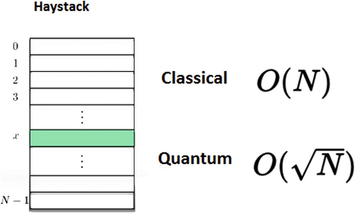
Unstructured search time complexities
- 1.
Prepare the input given f: {0, 1, … , N-1} → {0,1}. Note that the size of the input is 2n where n is the number of bits and N is the number of steps or size of the haystack. The ultimate goal is to find x such that f(x) = 1.
- 2.
Apply a basis superposition to all qubits in the input.
- 3.
Perform a phase inversion on the input qubits.
- 4.
Perform an inversion about the mean on the input.
- 5.
Repeat steps 3 and 4 at least
 times. There is a high probability that x will be found at this point.
Let’s take a closer look at the critical phase inversion and inversion about the mean steps.
Phase Inversion

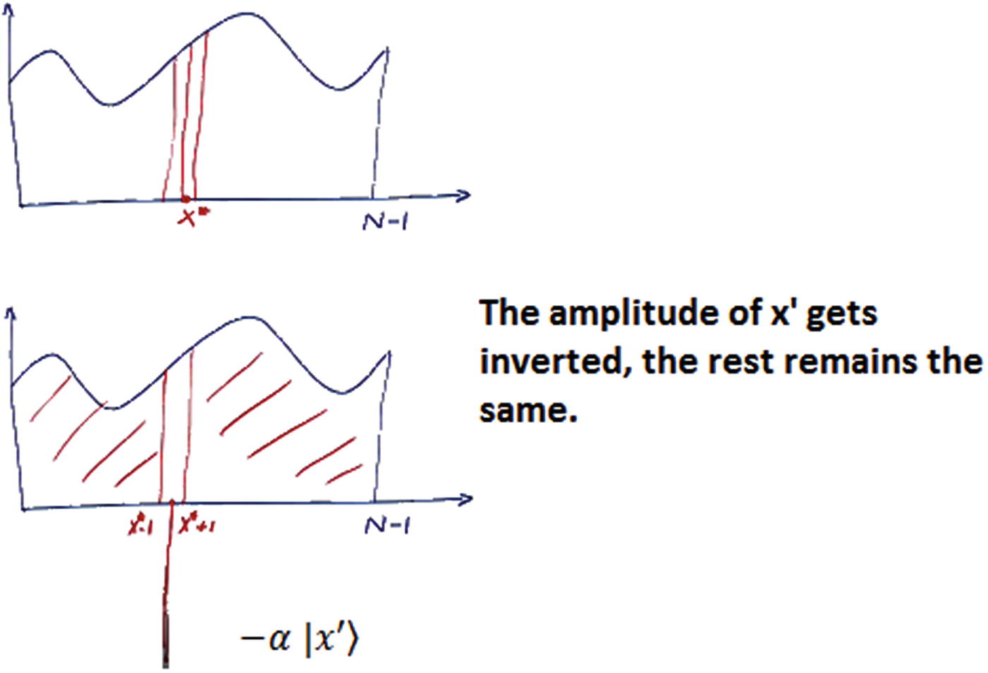
Pictorial representation of phase inversion
This is the first step in Grover’s algorithm; we’ll see how phase inversion helps on finding the element we are looking for, but for now let’s look at the second step: inversion about the mean.
Inversion About the Mean


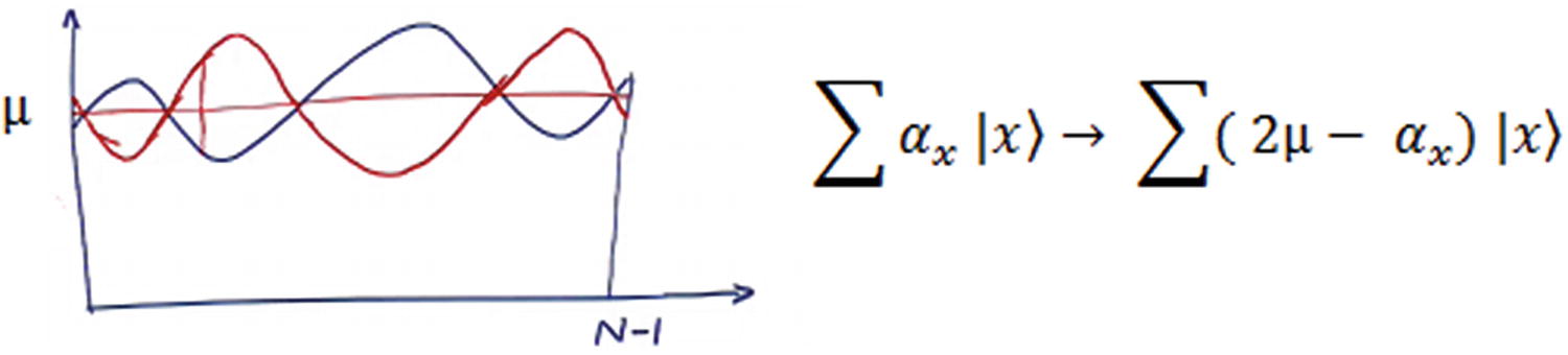
Graphical representation of inversion about the mean
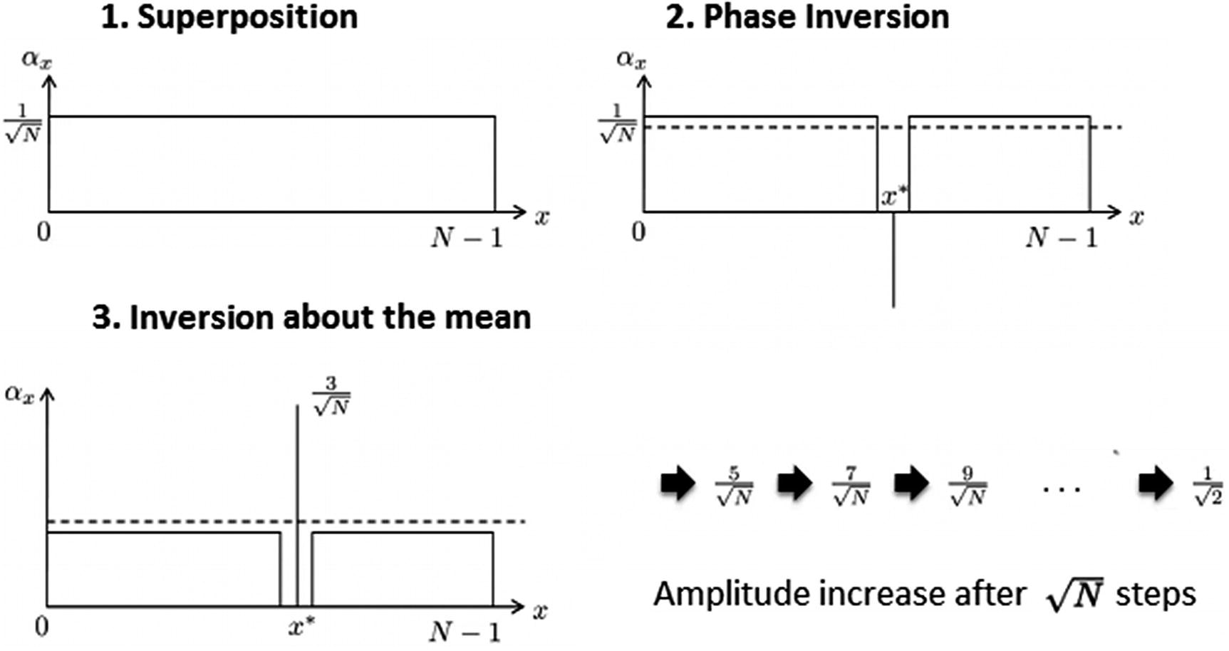
Single Grover’s iteration
The superposition of all qubits puts all amplitudes at
 .
.Next, a phase inversion puts the amplitude for xʹ at
 . Note that this has the effect of lowering slightly the value of the mean μ, as shown by the dotted line in Figure 8-4 step 2.
After the inversion about the mean, the mean amplitude drops a little bit, but xʹ goes way high, as much as
 above the mean μ.
If we repeat this sequence, the amplitude of x’ increases by about
 until that, in about
  steps, the amplitude becomes
  .
.At this point, if we measure our qubits, the probability of finding x’ (the element we are looking for), as defined by quantum mechanics, is the square of the amplitude. That is, ½.
Thus we are done. In roughly
 steps, we have found the marked element xʹ.
Now, let’s put all this together in a quantum circuit and corresponding code implementation.
Practical Implementation
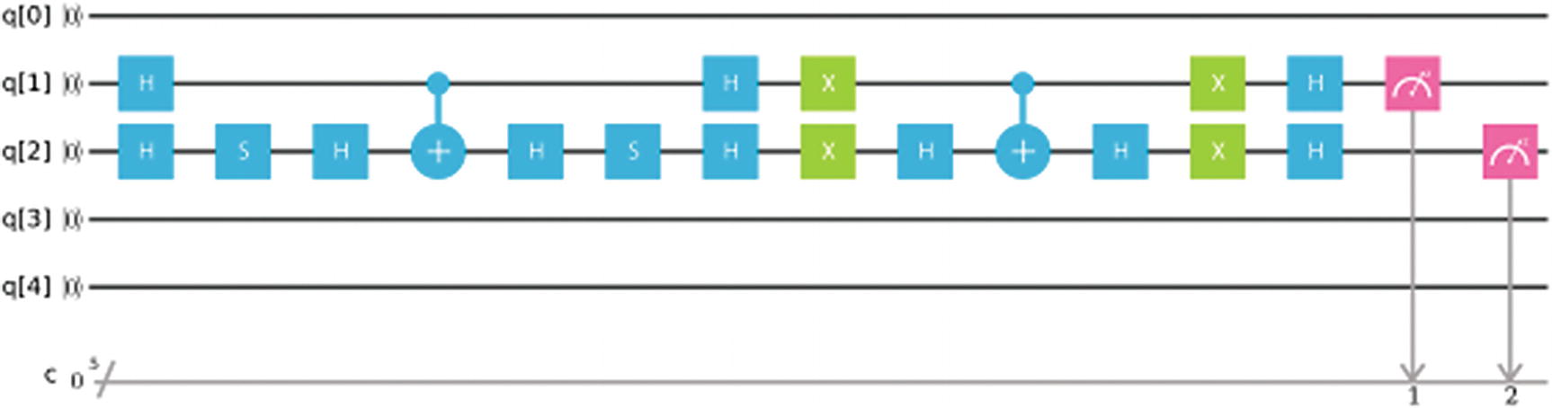
Quantum circuit for Grover’s algorithm with 2 qubits and A = 01
Python Script for Circuit in Figure 8-5
Listing 8-1 performs a single interaction of Grover’s algorithm for a 2-bit input using 2 qubits. Even though the pseudocode in the previous section states that the total number of iterations is given by roughly
 steps, the inversion about the mean requires this value to be multiplied by π/4 and its floor extracted (see the proof next to Figure 8-8). Therefore, we end up with
  where N = 2bits. Thus, for 2 bits we get
  .
.The script begins by creating a quantum circuit with 2 qubits and two classical registers to store their measurements.
Next, all qubits are put in superposition using the Hadamard gate.
Next, perform a phase inversion followed by an inversion about the mean on the input qubits corresponding to a single iteration of the algorithm.
Finally, measure the results and execute the circuit in the local or remote simulator. Print the result counts.
Generalized Circuit
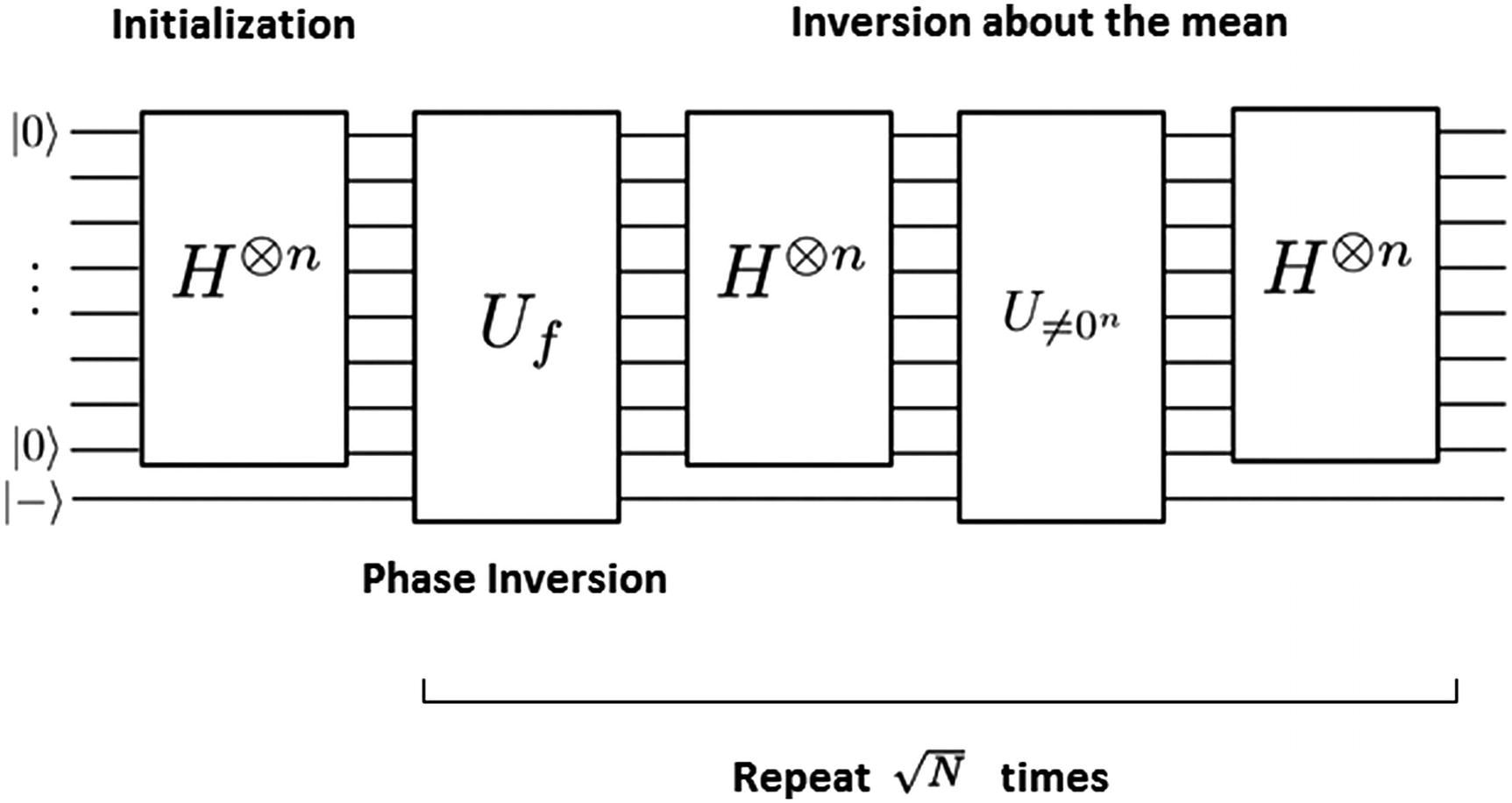
Generalization of Grover’s algorithm for an arbitrary number of qubits
The first box in Figure 8-6 puts all qubits in superposition by applying the Hadamard gate to the input of size n. This is the initialization step.
- Next, the phase inversion circuit (Uf) receives the superimposed input ψ = ∑ α ∣ x⟩ and a phase input (minus state). This has the desired effect of putting the phase exactly where we want it. Thus the output becomes ∑ α (−1)f(x) ∣ x⟩. But how can this be achieved? The answer is that, by applying an exclusive OR on the minus state input, we obtain the desired effect ∣b⟩ → ∣ f(x) ⊕ b⟩ as shown in Figure 8-7. The third row of the XOR truth table between f(x) and b (the right side of Figure 8-7) shows the phase inversion effect.
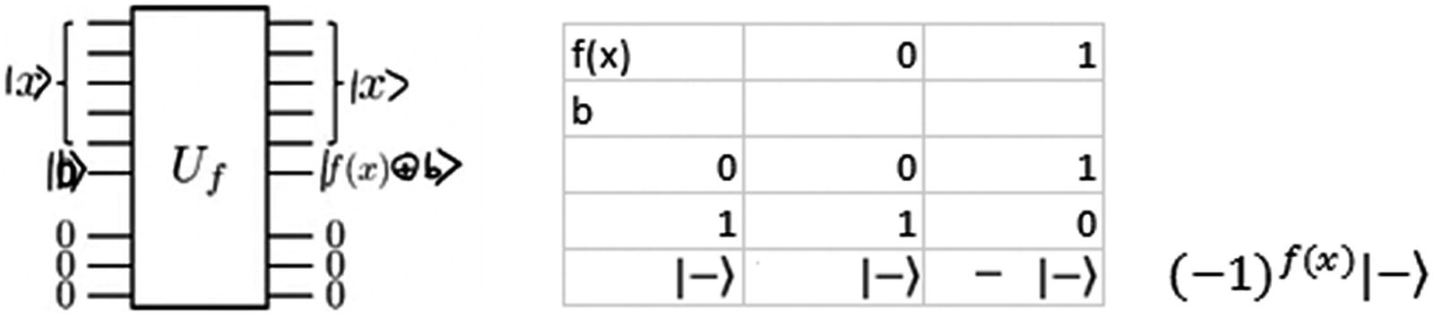 Figure 8-7
Phase inversion circuit
Finally, as shown in Figure 8-3, inversion about the mean is the same as doing the reflection about
 . To better visualize this, the superimposed state ψ and the mean μ can be represented as vectors over a 2D space as shown in Figure 8-8. To reflect ψ, create an orthogonal vector to μ, then project ψ over the new quadrant at the same angle θ.
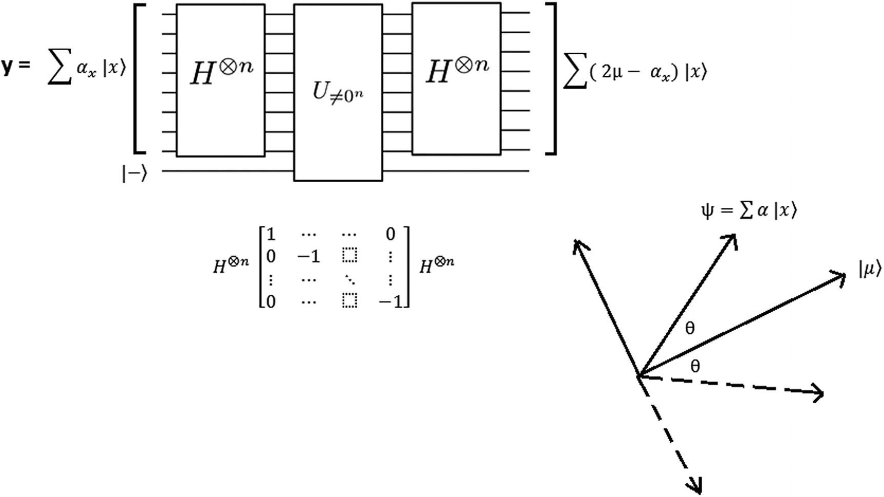
Inversion over the mean circuit
- 1.
Transform |μ> to the all zeros vector ∣0, …, 0⟩. This is achieved by applying the Hadamard gate to the input.
- 2.
Reflect about the all zeros vector ∣0, …, 0⟩. This can be done by multiplying it by the sparse matrix

- 3.
Transform ∣0, …, 0⟩ back to |μ> by applying the Hadamard again. Thus


 . Finally, applying matrix (1) to the state ψ = αx ∣ x⟩ yields
So this is Grover’s algorithm for unstructured search. It is fast, powerful, and soon to be hard at work on the data center cranking up all kinds of database searches. Given its significant performance boost over its classical cousin, chances are that in a few years, when quantum computers become more business friendly, most web searches will be performed by this quantum powerhouse. Before we finish, it is worth noting that, by the time of this writing, a useful implementation or experiment (one that can find a real thing) does not exist for IBM Q Experience. Hopefully this will change in the future, but for now Grover’s algorithm lives in the theoretical side of things. In the next section, we close strong by looking at the famous Shor’s algorithm for integer factorization.
Integer Factorization with Shor’s Algorithm
The game of cat and mouse between cryptography and crypto analysis rages on: the first, devising new ways to encrypt our everyday data, and the latter probing for weaknesses, always looking for a crack to bring it down. Current asymmetric cryptography relies on the well-known difficulty of factoring very large primes (in the hundreds of digits range). This section looks at the inner workings of Shor’s algorithm, a method that gives exponential speedup for integer factorization using a quantum computer. This is followed by an implementation using a library called ProjectQ. Next, we simulate for sample integers and evaluate the results. Finally we look at current and future directions of integer factorization in quantum systems. Let’s get started.
Challenging Asymmetric Cryptography with Quantum Factorization

where N is the number to factor and r is the period of x modulo N.
Tip
Large integer factorization is a problem that has puzzled mathematicians for millennia. In 1976, G. L. Miller postulated that using randomization, factorization can be reduced to finding the period of an element a modulo N, thus greatly simplifying this puzzle. This is the basic idea behind Shor’s algorithm.
- 1.
Input preparation: Done in a classical computer in polynomial time log (n).
- 2.
Find the period r of the element a such that ar ≡ 1 (mod N) via a quantum circuit. According to Shor, this takes O((log n)2(log log n)(log log log n)) steps on a quantum computer.
- 3.
Postprocessing: Done in a classical computer in polynomial time log (n).
Time Complexities for Common Factorization Algorithms
Algorithm | Time complexity |
|---|---|
Shor’s | (logn)2(log log n) (log log log n) |
Number Field Sieve |
|
Quadratic Sieve |
|


Incredibly, Shor’s algorithm has a polynomial time complexity, far superior to the exponential time by the Number Field Sieve, the fastest known method for factorization in a classical computer. As a matter of fact, experts have estimated that Shor’s could factor a 200+ digit integer in a matter of minutes. Such a feat would rock the foundation of current asymmetric cryptography used to generate the encryption keys for all of our web communications.
Tip
Symmetric cryptography is highly resistant to quantum computation and thus to Shor’s algorithm.
But don’t panic yet; a practical implementation in a real quantum computer is still a long way. Nevertheless, the algorithm can be simulated in a classical system using the slick Python library: ProjectQ. We’ll run ProjectQ’s implementation in a further section, but next let’s see how period finding can solve the factorization problem efficiently.
Period Finding
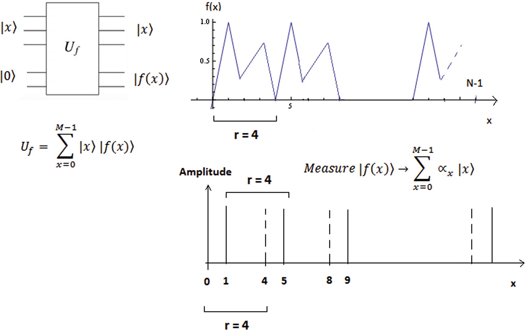
Periodic function f(x)
- 1.
f(x) is one-to-one on each period; that is, the values of f(x) must not repeat. In Figure 8-9 these values are represented by the vertices of each line per period.
- 2.
For any given M or the number of periods, r must divide M. For example, given M = 100 and the period r = 4, M/r = 25.
- 3.
M divided by r must be greater than r. That is, M > r2.
Shor’s algorithm transforms f(x) into a quantum circuit Uf where the inputs are in superposition. If we measure the second register in Uf, we may see values for the amplitudes  as shown in the amplitude chart of Figure 8-9. Here the amplitudes are exactly four units apart which is the period we are looking for. In this particular case, we get periodic superpositions with r = 4. But what do we do with this periodic superposition? Shor’s relies on another trick: Fourier sampling or quantum Fourier transform.
Fourier Sampling
It allows for input shifting without changing the output distribution.
This is good because now we have a periodic superposition where the non-zero amplitudes are the multiples of the period (see Figure 8-10).
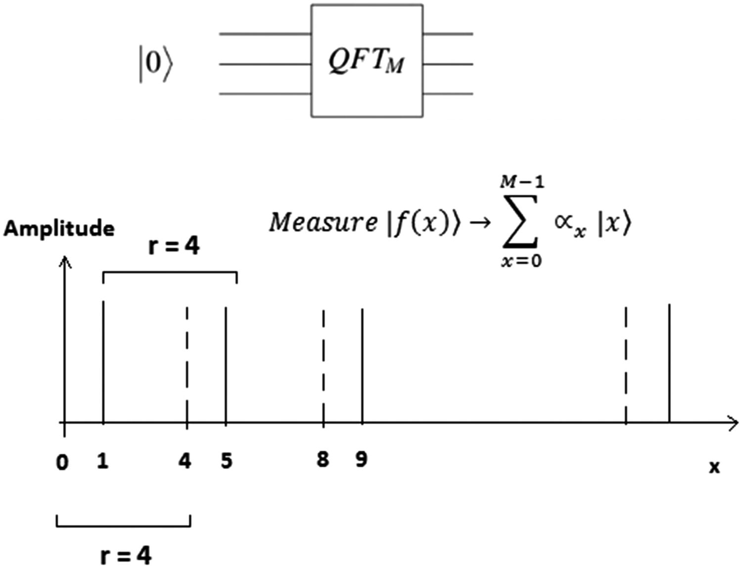
Fourier sampling showing periodic superposition
But what is the output of Fourier sampling? And how does it help? The answer is that its output is a random multiple of M/r. In this case given M = 100 and r = 4, we get a random multiple of 100/4 = 25. This is advantageous for our goal. Let’s see how.
Feed the Fourier Sampling Results to Euclid’s Greatest Common Divisor
If we were to run Fourier sampling multiple times, we will get random multiples of M/r. For example, we may get 50, 75, 25, etc. Now, if we apply Euclid’s greatest common divisor (gcd) to our random outputs, then viola: By dividing M by the gcd, we get the period r. Thus
r = M/gcd(50, 75, …) = 100 /25 = 4
Modular arithmetic: a = b (mod N). For example, 3 = 15 (mod 12).
Greatest common divisor gcd(a, b). For example, gcd(15, 21) = 3.
N divides (x +1) (x – 1).
N does not divide (x ± 1).
Finally, recover a prime factor by applying gcd(N, x+1).
In this case, 26 = (23)2. Thus 23 = 8 is a nontrivial factor such that 21 divides (8 + 1)(8 – 1). Finally we recover a factor with the greatest common divisor gcd (N, x+1) = gcd(21, 9) = 3. In general terms, pick an x at random, and then loop through x0, x1,…, xr ≡ mod N. If we are lucky, then r is even, that is, (xr/2)2 ≡ 1 (mod N). And thus we have a nontrivial square root of 1 mod N.
Tip
It has been proven that the probability that we get lucky, that is, r is even for x2 ≡ 1 (mod N), is ½. If we are unlucky, on the other hand, then we must repeat the procedure all over again. However given the high probability of success, this would be insignificant in the great scheme of things.
Now, let’s run the algorithm using the slick Python library ProjectQ.
Shor’s Algorithm by ProjectQ
- 1.
If N is even, return the factor 2.
- 2.
Classically determine if N = pq for p ≥ 1 and q ≥ 2, and if so, return the factor p (in a classical computer, this can be done in polynomial time).
- 3.
Choose a random number a, such that 1 < a ≤ N – 1. Using Euclid’s greatest common divisor, determine if gcd (a, N) > 1. If so, return the factor gcd(a, N).
- 4.
Use the order-finding quantum circuit to find the order r of a modulo N. In a quantum computer, this step is done in polynomial time.
- 5.
If r is odd or r is even but ar/2 = –1 (mod N), then go to step 3. Otherwise compute gcd(ar/2 – 1, N) and gcd(ar/2 + 1, N). Test to see if one of these is a nontrivial factor of N, and return the factor if so (in a classical computer, this can be done in polynomial time).
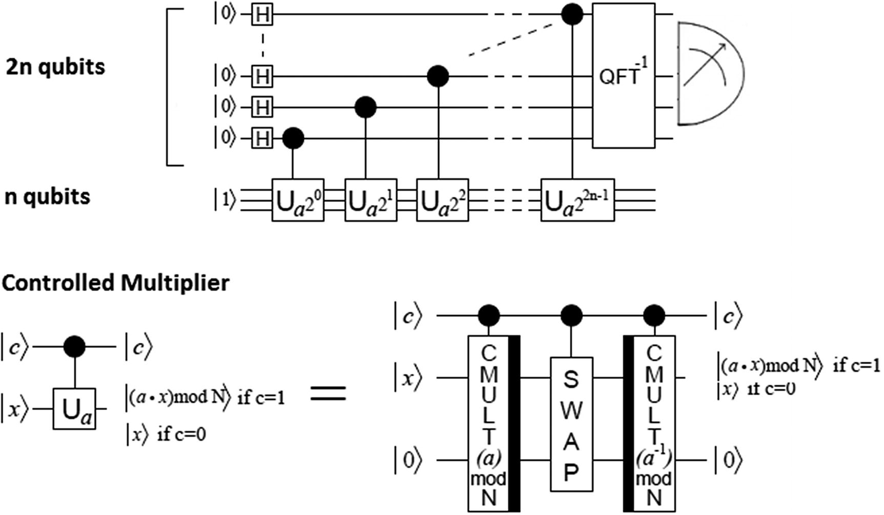
Beauregard quantum circuit for period finding
- A controlled multiplier Ua maps ∣x⟩ → ∣ ax (mod N)⟩ where
a is a classical relative prime to use as the base for ax (mod N).
x is the quantum register.
c is the register of control qubits such that Ua = ax (mod N) if c =1 and x otherwise.
- The controller multiplier Ua is in turn implemented as a series of doubly controlled modular adder gates such that
If both control qubits c1 = c2 = 1, the output is f(x) = ∣ φ(a+b mod N)⟩. That is, a + b (mod N) in Fourier space. Note that this gate adds two numbers: a relative prime (a) and a quantum number (b).
If either control qubit (c1, c2) is in state |0>, then f(x) = ∣ φ(b )⟩.
The doubly controlled modular adder gate is in turn built on top of the quantum addition circuit by Draper3. This circuit implements addition of a classical value (a) to the quantum value (b) in Fourier space.
Factorization with ProjectQ
Shor’s Algorithm by ProjectQ in Action
The number of qubits used: Given N = 21 we need 5 bits; thus total-qubits = 2 * 5 + 3 = 13.
The total number of gates used by type: In this case, doubly controlled CCR = 1467, CR = 7180, CSwap = 50, CX = 200, R = 608, X = 206, and others, for a grand total of 12,646 quantum gates.
- The run_shor function takes three arguments:
The quantum engine or simulator provided by ProjectQ plus
N: The number to factor
a: The relative prime to use as a base for ax mod N
The function then loops from a = 0 to a = ln(N) with the quantum input register x in superposition; it then performs the quantum circuit for f(a) = ax mod N as shown in Figure 8-11.
Next, it performs Fourier sampling on the x register conditioned on previous outcomes and performs measurements.
Finally it sums the measured values into a number in range [0,1]. It then uses continued fraction expansion to return the denominator or potential period (r).
ProjectQ Period Finding Quantum Subroutine
The next section compiles a set of factorization results for various values of N.
Simulation Results
Factorization Results for Various Values of N
Number (N) | Qubits | Time (s) | Memory (MB) | Quantum gate counts |
|---|---|---|---|---|
15 | 11 | 2.44 | 50 | CCR = 792 CR = 3186 CSwap = 32 CX = 128 H = 1408 R = 320 X = 130 Measure = 9 |
105 | 17 | 27.74 | 200 | CCR = 3735 CR = 25062 CSwap = 98 CX = 392 H = 6666 R = 1568 X = 393 Measure = 15 |
1150 | 25 | 17542.12 (4.8 h) | 500 | CCR = 15366 CR = 139382 CSwap = 242 CX = 968 H = 24222 R = 5829 X = 981 Measure = 23 |
2491 | 27 | 246164.74 (68.3 h) | 2048 | CCR = 20601 CR = 194670 CSwap = 288 CX = 1152 H = 31126 R = 7509 X = 1166 Measure = 25 |
Factorizing the four-digit number 2491 took more than 68 hours on a 64-bit Windows 7 PC with an Intel Core i-5 CPU at 2.6 GHz with 16 GB of RAM. I tried to go a bit higher by attempting to factorize N = 8122 but gave up after one week. All in all, these results show that the algorithm can be simulated successfully for small numbers of N; however it needs to be implemented in a real quantum computer to test its real power.
This chapter brought proceedings to a close with two algorithms that have generated excitement about the possibilities of practical quantum computation: Grover’s algorithm, an unstructured quantum search method capable of finding inputs at an average of square root of N steps. This is much faster than the best classical solution at an average of N/2 steps. Expect all web searches to be performed by Grover’s algorithm in the future.
Shor’s algorithm for factorization in a quantum computer which experts say could bring current asymmetric cryptography to its knees. Shor’s, arguably the most famous quantum algorithm out there, is a prime example of the power of quantum computation by providing exponential speedups over the best classical solution.
Finally, I would like to close things up by saying that I have tried my best to explain the difficult concepts of quantum computing by mixing math, software, and as many figures I can muster. A lot of coffee cups and sleepless nights were spent writing this manuscript, not to mention that I find most of the math as confusing as you probably do. I hope you enjoy reading this book as much as I did writing it, and remember: The great physicist Richard Feynman once said “If somebody tells you that he understands Quantum Mechanics it means he doesn’t understand Quantum Mechanics.”