Chapter 2. Diving into Data Programming with Snorkel
Before the advent of Deep Learning, data scientists would spend most of their time on feature engineering: working to craft features that enabled models to perform better on some metric of choice. Deep Learning, with its ability to discover features from data, has freed data scientists from feature engineering, and shifted their efforts towards other tasks like understanding the selected features, hyperparameter tuning, and robustness checks.
With the recent advent of the “Deep Learning era”, data engineering has rapidly become the most expensive task in terms of both time and expense. This task is particularly time consuming for scenarios where data is not labeled. Enterprises gather a lot of data, but a good part of that is unlabeled data. Some enterprise scenarios, like advertising, naturally enable gathering raw data and their labels at the same time. To measure whether the advertising presented to the user was a success or not, for instance, a system can log data about the user, the advertisement shown, and whether the user clicked on the link presented, all as one record of the dataset. Associating the user profile with this data record creates a ready-to-use labelled dataset.
However applications such as email, social media, conversation platforms, etc., produce data that cannot be easily associated with labels at the time the dataset is created. To make this data usable, machine learning practitioners must first label the data, often via processes that are time-consuming and scale linearly with the size of the unlabeled data.
Tackling the data labelling process is at the heart of weak supervision. In this chapter we will focus on data programming techniques for weak supervision offered by the Snorkel software package
Snorkel, a data programming framework
Snorkel is a framework that implements easy-to-use, modern solutions for key data engineering operations like data labeling and data augmentation through a lens called “data programming.” For data labeling, practitioners can encode the heuristics they use to classify samples of data to different categories using standard software tools, leverage state-of-the-art statistical modeling techniques to estimate the accuracies of these heuristics, and programmatically create “weakly labeled” data by applying those heuristics to unlabeled data and aggregating their signal using the learned statistical model.
For data augmentation, Snorkel allows data engineers to amplify limited datasets by generating new samples that respect known invariances, ensuring that models trained on the resulting data are able to do the same.
To install Snorkel, simply use pip:
pipinstallsnorkel
Looking at the contents of the Snorkel package, you will notice that the main sub-packages are:
-
Labeling - tools to generate labels for the data, and reconcile those labels generating a single one at the end.
-
Analysis - utilities to calculate metrics evaluating labeling.
-
Augmentation - tools that help generate new data samples.
-
Slicing - tools to monitor how a subset of data, with particular characteristics, has affected the training.
-
Classification - tools to train multi-task models.
In the rest of this chapter, we will dive deeper into how to leverage the labeling, analysis, and augmentation subpackages for our data programming needs. Although we will not cover the “Slicing” package, we recommend getting familiar with it. The Snorkel.org site has a really good tutorial on it.
Let’s get labeling!
Getting started with Labeling Functions
In Snorkel, “labeling functions” encode the rules that the data engineers or domain experts follow to assign each sample of data to a particular class. Labeling functions may be written in any number of ways, but the most common is via simple Python snippets.
The best way to get started creating labeling functions is to get to know subsets of data that share properties that provide signal for the problem of interest. You can then proceed to create functions that:
-
test each data sample for those properties
-
for a classification problem (which we’ll focus on here) either “vote” to assign the data point to one of the classes or abstain.
Intuitively, you can think of each labeling function as a weak classifier that operates over some subset of the data. Typically, you would want to create several labeling functions for any given problem. These labeling functions can be noisy, correlated, and use whatever external resources might be useful; the statistical modeling behind Snorkel will do the heavy lifting to aggregate the signal from the labeling functions into weak labels for each data point.
Let us get practical about how to use Snorkel.Suposee we wish to train a classifier that attempts to determine whether integers are prime or not. To train, we need labeled examples: pairs of integers and their corresponding prime/not prime tags. However, we only have an unlabeled set of data. Our goal, with Snorkel, is to create a set of labels by writing labeling functions. Next we show a set of examples for this scenario.
data=[5,21,1,29,32,37,10,20,10,26,2,37,34,11,22,36,12,20,31,25]df=pd.DataFrame(data,columns=["Number"])
The code above creates an array of 20 integers, data. It then initializes a Pandas DataFrame with a single column named “Number”, and the values of the data array as records.
Next let’s establish our convention of which numeric labels will correspond to the prime numbers, and which to the non-prime numbers.
ABSTAIN=-1NON_PRIME=0PRIME=1
As you can see, besides the PRIME and Non_Prime labels, we have introduced a third option ABSTAIN. ABSTAIN will be used when none of the rules encoded seems to match the data point that is being analyzed. Note that the ABSTAIN option has important (and positive!) implications for the ability of Snorkel’s statistical modeling techniques to estimate labeling function’s accuracy.
The next step is to define our “labeling functions”. Here, our labeling functions are regular Python functions that contain logic indicating whether:
-
a given sample is prime
-
an example is not prime
-
unclear based on the logic coded by the function (ABSTAIN).
What makes a given Python function a labeling function in code, is the @labeling_function() decorator. The argument passed to the decorator is the dataset row.
For our prime/non-prime labeling problem, one of the labeling functions could encode whether a number is odd or even”. If the number is even, the function will vote for this record to not be a prime number. This logic is not complete, because the number 2 is even, and is prime as well, but it also is the only even prime, and the Snorkel labelers do not need to be perfect; they only need to be better than random chance. Recall further that each labeling function can provide signal on some subset of the data and abstain for the remainder, allowing other labeling functions to handle the uncovered portion
First, let’s import the package containing the definition of the labeling function decorators:
fromsnorkel.labelingimportlabeling_function
Next let’s code the is_even labeling function, as we described it above.
@labeling_function()defis_even(record):ifrecord["Number"]%2==0:returnNON_PRIMEelse:returnABSTAIN
Another labeling function can be is_odd. As the name suggests, this function can check whether the number is odd, and if not, suggest that it is not a prime number.
Note
The logic of the is_even function, is identical to the logic of the is_odd function, and we should not use two identical functions, in practice. Those two functions are used here just to illustrate that Snorkels can successfully deal with highly correlated labeling functions.
The logic for the is_odd function would be:
@labeling_function()defis_odd(record):ifrecord["Number"]%2==1:returnABSTAINelse:returnNON_PRIME
Another labeling function can be one that “knows” that number 2 is a prime number, as illustrated in the sample below:
@labeling_function()defis_two(record):ifrecord["Number"]==2:returnPRIMEelse:returnABSTAIN
The final labeling function we will use, encodes “knowing” that some specific numbers are prime, and it only votes for those ones to be PRIME, abstaining for all other numbers. Let’s call this function: is_known_prime.
#The list of "known" prime numbersknown_primes=[2,3,5,7,11,13,17,19,23,29]@labeling_function()defis_known_prime(record):ifrecord["Number"]inknown_primes:returnPRIMEelse:returnABSTAIN
Now that we have our labeling functions, we will proceed to use them on the dataset.
Applying the labels to the datasets
The process of getting the labeling functions to “vote” on each record is called “applying the labeling functions”. The family of objects that applies the labeling functions is called appliers. There are several appliers:
-
DaskLFApplier- Applies the defined labeling functions to the Dask DataFrames (Dask is a DataFrame composed of smaller Pandas DataFrames that are accessed and operated upon in parallel). -
PandasLFApplier- Applies the array of labeling functions to a Pandas data frame. -
PandasParallelLFApplier- This applier operates by parallelizing the Pandas data frame into a Dask data frame and uses theDaskLFApplierto work on the partitions in parallel, being, therefore, faster than thePandasLFApplier. -
SparkLFApplier- Applies the labeling functions over a Spark Resilient Distributed Dataset(RDD).
For our example, since the data is small and the process can easily run on a desktop or laptop, we will be using the PandasLFApplier.
Let’s import the Snorkel PandasLFApplier.
fromsnorkel.labelingimportPandasLFApplier
Next, let’s define an array, lfs where we will declare all the labeling functions, followed by the applier PandasLFApplier.
The applier.apply call applies the labeling functions to the data frame df.
lfs=[is_odd,is_even,is_two,is_known_prime]applier=PandasLFApplier(lfs=lfs)L_train=applier.apply(df=df)
Analyzing the labeling performance
After applying the labeling functions, we can run an analysis on how they are performing. Snorkel comes equipped with LFAnalysis which summarizes the performance of the labeling functions by describing: polarity, coverage, overlaps, and conflicts.
To make use of LFAnalysis let us start with importing the package, and then printing the LFAnalysis summary.
fromsnorkel.labelingimportLFAnalysisLFAnalysis(L=L_train,lfs=lfs).lf_summary()
The output is a pandas data frame summarizing the four metrics above.
| Number | j | Polarity | Coverage | Overlaps | Conflicts |
|---|---|---|---|---|---|
is_odd |
0 |
[0] |
0.55 |
0.55 |
0.05 |
is_even |
1 |
[0] |
0.55 |
0.55 |
0.05 |
is_two |
2 |
[1] |
0.05 |
0.05 |
0.05 |
is_known_prime |
3 |
[1] |
0.20 |
0.05 |
0.05 |
Polarity
Polarity shows which labels each labeling function has emitted when evaluated over a given set of data (note that ABSTAIN is not considered a label). Polarity is therefore 0 for is_odd and is_even, because those functions are built to either ABSTAIN or return NON_PRIME (we defined NON_PRIME = 0), while for is_two and is_known_prime polarity is 1 because those two functions are build to either ABSTAIN or return PRIME (PRIME = 1).
When would looking at the Polarity come in particularly handy? Imagine we had a labeling function that was expected to return both classes — e.g. 0 and 1 — but the observed Polarity is only 0. This could indicate an error in the logic that returns class 0, so we should check for any potential bugs. If there are no bugs, it might also be worth double-checking our reasoning around that logic, as we are not obtaining the expected empirical results.
The polarity itself can also be retrieved through the lf_polarities() call.
LFAnalysis(L=L_train,lfs=lfs).lf_polarities()
[[0], [0], [1], [1]]
Coverage
For each labeling function, the Coverage characteristic indicates what fraction of the data the labeling function did not abstain for, and returned one of the other values. In other words, coverage is a measure of how often your labeling functions have opinions about examples in the datasets.
| Coverage | |
|---|---|
is_odd |
0.55 |
is_even |
0.55 |
is_two |
0.05 |
is_known_prime |
0.20 |
To understand the values presented by Coverage, we can apply each labeling function to the data frame, and inspect the results.
df["is_odd"]=df.apply(is_odd,axis=1)df["is_even"]=df.apply(is_even,axis=1)df["is_two"]=df.apply(is_two,axis=1)df["is_known_prime"]=df.apply(is_known_prime,axis=1)
The output will be in the following data frame.
| Number | is_odd | is_even | is_two | is_known_prime |
|---|---|---|---|---|
5 |
-1 |
-1 |
-1 |
1 |
21 |
-1 |
-1 |
-1 |
-1 |
1 |
-1 |
-1 |
-1 |
-1 |
29 |
-1 |
-1 |
-1 |
1 |
32 |
0 |
0 |
-1 |
-1 |
37 |
-1 |
-1 |
-1 |
-1 |
10 |
0 |
0 |
-1 |
-1 |
20 |
0 |
0 |
-1 |
-1 |
10 |
0 |
0 |
-1 |
-1 |
26 |
0 |
0 |
-1 |
-1 |
2 |
0 |
0 |
1 |
1 |
37 |
-1 |
-1 |
-1 |
-1 |
34 |
0 |
0 |
-1 |
-1 |
11 |
-1 |
-1 |
-1 |
1 |
22 |
0 |
0 |
-1 |
-1 |
36 |
0 |
0 |
-1 |
-1 |
12 |
0 |
0 |
-1 |
-1 |
20 |
0 |
0 |
-1 |
-1 |
31 |
-1 |
-1 |
-1 |
-1 |
25 |
-1 |
-1 |
-1 |
-1 |
If we look at one of the labeling functions, the is_odd, for example, has returned a value different from ABSTAIN (NON-PRIME) for 11 out of 20 records. That is why the coverage for this labeling function is 11/20, or 0.55.
| Number | is_odd | is_even | is_two | is_known_prime |
|---|---|---|---|---|
32 |
0 |
0 |
-1 |
-1 |
10 |
0 |
0 |
-1 |
-1 |
20 |
0 |
0 |
-1 |
-1 |
10 |
0 |
0 |
-1 |
-1 |
26 |
0 |
0 |
-1 |
-1 |
2 |
0 |
0 |
1 |
1 |
34 |
0 |
0 |
-1 |
-1 |
22 |
0 |
0 |
-1 |
-1 |
36 |
0 |
0 |
-1 |
-1 |
12 |
0 |
0 |
-1 |
-1 |
20 |
0 |
0 |
-1 |
-1 |
The coverage can also be retrieved through the lf_coverages() call.
LFAnalysis(L=L_train,lfs=lfs).lf_coverages()
array([0.55, 0.55, 0.05, 0.2 ])
The coverage of the labeling functions should match your expectations about the distribution of the characteristics used by each labeling function in your validation data. If you encode a rule thinking that it should not abstain for 30% of the data, and you see it covering 90% of the data, it is time to check the logic of the labeling function or examine your expectations.
Overlaps
The Overlaps metric is a measure of often two labeling functions vote on the same points. Concretely, it indicates what fraction of the data non-ABSTAIN return values from one labeling function have overlapped with non-ABSTAIN return values from another labeling function. Practically, as you can see above in the Table 2-4 table, the is_known_prime function has returned a PRIME value 4 out of 20 times; for numbers: 5, 29, 2, 11. It has ABSTAIN-ed for all other records.
| Number | is_odd | is_even | is_two | is_known_prime |
|---|---|---|---|---|
5 |
-1 |
-1 |
-1 |
1 |
29 |
-1 |
-1 |
-1 |
1 |
2 |
0 |
0 |
1 |
1 |
11 |
-1 |
-1 |
-1 |
1 |
As we can see from the table above, for those same four records, only in the case of number 2 the other labeling functions have emitted a 0 or a 1. is_known_prime has overlapped only once with another labeling function, 1/20, therefore its measure is 1/20, or 0.05.
| Number | Overlaps |
|---|---|
is_odd |
0.55 |
is_even |
0.55 |
is_two |
0.05 |
is_known_prime |
0.05 |
The calculations are the same for the other labeling functions. If we look back at the table, the is_odd and is_even both overlap with each other or the other two functions 11/20 times, or 0.55.
The Overlaps can also be calculated through the lf_overlaps() call.
LFAnalysis(L=L_train,lfs=lfs).lf_overlaps()
array([0.55, 0.55, 0.05, 0.05])
Conflicts
Conflicts indicate the fraction of the data in which this labeling function’s non-abstaining decision has conflicted with another labeling function’s non-abstaining decision.
| Conflicts | |
|---|---|
is_odd |
0.05 |
is_even |
0.05 |
is_two |
0.05 |
is_known_prime |
0.05 |
We can see that for each labeling function, that ratio seems to be 0.05 or 1/20 samples. Inspecting the data frame presented in Table 2-3, where we put together the output of each labeling function in a column, we can see that there is a single record that has some disagreement between all labeling functions. This record is behind the 0.05 conflicts statistics.
| Number | is_odd | is_even | is_two | is_known_prime |
|---|---|---|---|---|
2 |
0 |
0 |
1 |
1 |
Labeling functions that conflict significantly with other labeling functions may be useful so long as they are not worse than random chance; otherwise, they might need a more careful look.
The Conflicts can also be calculated through the lf_conflicts() call.
LFAnalysis(L=L_train,lfs=lfs).lf_conflicts()
array([0.05, 0.05, 0.05, 0.05])
Using a validation set
Let us assume that for a small portion of the data we have ground truth labels. This data can serve as a validation set. Even when we do not have a validation set, it often is possible to label a subset of the data using subject-matter experts (SMEs). Having this validation dataset (10% - 20% the size of the training data, depending on how representative of the entire dataset you think that portion is) can help evaluate further the labelers. On this set, we can calculate the additional statistics: “Correct”, “Incorrect” and “Empirical Accuracy”.
To make use of the validation set, we would start by applying the labeling functions to it.
# define a validation set, and create a DataFramevalidation=[22,11,7,2,32]df_val=pd.DataFrame(validation,columns=["Number"])# gather the ground truth labelstrue_labels=np.array([0,1,1,1,0])# apply the labelsL_valid=applier.apply(df_val)# analyze the labelers and get the summary dfLFAnalysis(L_valid,lfs).lf_summary(true_labels)
The resulting data frame will have the additional three-column statistics, from the initial one presented in Table 2-9: Correct, Incorrect, Empirical Accuracy.
| j | Polarity | Coverage | Overlaps | Conflicts | Correct | Incorrect | Emp. Acc. | |
|---|---|---|---|---|---|---|---|---|
is_odd |
0 |
[0] |
0.6 |
0.6 |
0.2 |
2 |
1 |
0.666667 |
is_even |
1 |
[0] |
0.6 |
0.6 |
0.2 |
2 |
1 |
0.666667 |
is_two |
2 |
[1] |
0.2 |
0.2 |
0.2 |
1 |
0 |
1.000000 |
is_known_prime |
3 |
[1] |
0.6 |
0.2 |
0.2 |
3 |
0 |
1.000000 |
The “Correct” and “Incorrect” are the actual count of samples this labeling function has correctly or incorrectly labeled. It is easier to interpret these numbers by looking at the output of the labeling functions. Doing this, of course, is just for this illustration, as it does not scale in practice.
df_val=pd.DataFrame(validation,columns=["Number"])df_val["is_odd"]=df_val.apply(is_odd,axis=1)df_val["is_even"]=df_val.apply(is_even,axis=1)df_val["is_two"]=df_val.apply(is_two,axis=1)df_val["is_known_prime"]=df_val.apply(is_known_prime,axis=1)df_val
| Number | is_odd | is_even | is_two | is_known_prime | ground_truth |
|---|---|---|---|---|---|
22 |
0 |
0 |
-1 |
-1 |
0 |
11 |
-1 |
-1 |
-1 |
1 |
1 |
7 |
-1 |
-1 |
-1 |
1 |
1 |
2 |
0 |
0 |
1 |
1 |
1 |
32 |
0 |
0 |
-1 |
-1 |
0 |
“Empirical Accuracy” is the percentage of samples that have been labelled correctly, ignoring samples on which the labeling function abstained. For is_known_prime, we can see that it has returned PRIME for three samples, and they have all been correct, therefore its Empirical Accuracy is 1.0. The is_even function, on the other hand, has been correct for 2/3 non-ABSTAIN returns, therefore its accuracy is 67%.
Reaching labeling consensuswith LabelModel
After creating the labeling functions and making use of the statistics to check on our assumptions and debug them, it is time to apply them to the dataset. In the process, for each record, we will get several “opinions”, one from each labeling function (unless one is abstaining) regarding which class a given example should belong to. Some of those class assignments might be conflicting, therefore we need a way to resolve the conflicts in order to assign a final label. To reach to this single label conclusion, Snorkel provides the LabelModel class.
The LabelModel learns a model over the predictions generated by the labeling functions using advanced unsupervised statistical modeling, and uses the predictions from this model to assign a probabilistic weak label to each datapoints.
label_model=LabelModel()label_model.fit(L_train=L_train,n_epochs=200,seed=100)preds_train_label=label_model.predict(L=L_train)preds_valid_label=label_model.predict(L=L_valid)L_valid=applier.apply(df_val)LFAnalysis(L_valid,lfs).lf_summary()preds_train_labelingModel=label_model.predict(L=L_train)preds_valid_labelingModel=label_model.predict(L=L_valid)df["preds_labelingModel"]=preds_train_labelingModel
| Number | preds_labelingModel | is_odd | is_even | is_two | is_known_prime |
|---|---|---|---|---|---|
5 |
1 |
-1 |
-1 |
-1 |
1 |
21 |
-1 |
-1 |
-1 |
-1 |
-1 |
32 |
0 |
0 |
0 |
-1 |
-1 |
2 |
0 |
0 |
0 |
1 |
1 |
The LabelModel estimates the accuracy of each labeling function given the particular labeling function’s predictions and how they relate to the out put of all other labeling functions. Those estimates are used as the parameters of the LabelModel which learns to predict a single label. The relationship between the labeling functions and the latent true label is modeled as a graphical model, shown in Figure 2-1. The LabelModel class estimates the parameters of this graphical model each time it is fit.

Figure 2-1. The labeling functions graphical model
Intuition behind LabelModel
The agreement and disagreement of the labeling functions serve as the source of information to calculate the accuracies of the labeling functions. The label model combines these agreements and disagreements with a type of independence—conditional independence, to obtain certain relationships that enable solving for the accuracies. The intuition behind why this is possible relates to the fact that if we have enough labeling functions, even just examining the most popular vote will provide a noisy, but higher-quality, estimate of the true label. Once this has been obtained, we can examine how each labeling function performs against this label to get an estimate of its accuracy. The actual functionality of the label model avoids this two-step approach and instead uses an application of the law of total probability and Bayes’ rule. Given conditional independence of the labeling functions S1, S2, it holds that
P(S1,S2) = P(S1, S2,Y=-1) + P(S1, S2,Y=+1)
= P(S1, S2 | Y=-1)P(Y=-1) + P(S1, S2 | Y=+1)P(Y=+1)
= P(S1|Y=-1)P(S2|Y=-1)P(Y=-1) + P(S1|Y=+1)P(S2 | Y=+1)P(Y=+1)
The left-hand side contains the agreement/disagreement rate between the two labeling functions, while the last equation contains the sum of products of accuracies (and the priors P(Y)).
Now, we can obtain at least two more such equations by adding additional labeling functions. We can then solve for the accuracy terms such as P(S1|Y=-1), either via gradient descent, or by solving a system of equations.
LabelModel parameter estimation
Above we provided some of the intuition behind how Snorkel obtains the accuracy parameters from agreements and disagreements among a few labeling functions. This can be generalized into an algorithm to obtain all of the accuracies. There are several such algorithms; the one used in Snorkel is described in more depth in Ratner et al. (Ratner et al. 2018).
As we saw, the key requirement was having conditional independence between labeling functions. A useful tool to represent the presence of such independences is a graphical model. These are graphical representations of dependence relationships between the variables, which can be used to obtain valid equations with the form described above. Remarkably, the graph structure also relates to the inverse of the covariance matrix between the labeling functions and the latent label node, and this relationship enables a matrix-based approach to solving for the accuracy parameters.
Specifically, it is possible to complete the inverse of the covariance matrix just based on the agreement and disagreement rates between the labeling functions. Having done this, we have access to the accuracies - the off-diagonal blocks of this covariance matrix - and can then better synthesize the labeling function votes into probabilistic labels using the graphical model formulation.
To illustrate the intuition about learning the probability of the accuracy of each labeling function with an example based on agreement/disagreement, let us image that we want to solve the following classification problem: separating a set of images into indoor and outdoor categories. Let us also assume that we have three labeling functions recognizing features related to the sky, clouds, and wooden floor. The labeling function describing the sky features, and the labeling function describing the clouds will probably agree in most pictures on whether the picture is indoor or outdoor, and have the opposite prediction with a labeling function judging whether there is a wooden floor in the picture. For datapoints we will have a data frame like the one represented in the table below:
| image | has_sky | has_clouds | has_wodden_floor |
|---|---|---|---|
indoor0 |
1 |
1 |
0 |
indoor1 |
1 |
1 |
0 |
indoor2 |
1 |
1 |
0 |
outdoor3 |
0 |
0 |
1 |
outdoor4 |
0 |
0 |
1 |
outdoor5 |
1 |
0 |
1 |
To train a LabelModel on this DataFrame, we would do:
L=np.array(df[["has_sky","has_clouds","has_wooden_floor"]])label_model=LabelModel()label_model.fit(L)np.round(label_model.get_weights(),2)
When you examine the weights of the label_model for each classification source (labeling function), you will notice how the first labeling function has_sky is weighted less than the second one, has_clouds due to the mistake it makes on data point “outdoors5”:
array([0.83, 0.99, 0.01])
The calculated conditional probabilities for each source and each class (outdoor, indoor, abstain) are retrieved via:
np.round(label_model.get_conditional_probs(),2)
And the actual conditional probability values placed in a matrix with dimensions [number of labeling function, number of labels + 1(for abstain), number of classes], rounded are:
array([[[0.  , 0.  ],
        [0.66, 0.01],
        [0.34, 0.99]],

       [[0.  , 0.  ],
        [0.99, 0.01],
        [0.01, 0.99]],

       [[0.  , 0.  ],
        [0.01, 0.99],
        [0.99, 0.01]]])
Strategies to improve the labeling functions
The “Interactive Programmatic Labeling for Weak Supervision” published at KDD, 2019 contains various suggestions on how to iteratively improve the labeling functions. One such suggestion is to focus on the data points where most of the labeling functions abstain, or conflict, and look for potential additional patterns. These suggestion are called the “abstain-based” and “disagreement-based” strategies. If you have identified a series of high-accuracy labeling functions, the next step would be to attempt to maximize the coverage from those labelers. If instead you are dealing with low accuracy labeling functions, the focus should be instead on how the ties are broken.
A more focused strategy suggested in the same paper, partitions the data based on patterns observed in it, and attempts to create labeling functions that should return a non-abstain value for the samples in the partition they are designed for, abstaining otherwise. Indicators of the quality of each labeling function are:
-
having a high fraction of data in the partition for which the labeling function returns one of the classes, referred in this paper as the IF - the Inside partition Fire rate.
-
have a low OF - outside partition fire rate, meaning the labeling functions returning a non-abstain value in the partitions other than the ones they were designed for
-
having an overall low FF- False Fire rate - the case when the labeling functions return the wrong class.
Data Augmentation with Snorkel Transformers
To this point in the chapter, we have focused on how to take advantage of Snorkel data programming techniques to label data using a combination of unlabeled data, human domain expertise encoded in heuristics, and unsupervised statistical modeling. We will now discuss how another set of techniques in Snorkel can be used to further increase the effective size of datasets for machine learning. Specifically, in addition to labeling existing data, we can synthetically generate training data by combining existing data points with transformations to which the task should be invariant. As an example, in Computer Vision problems, some well-known transformations include rotation, occlusion, brightness variation, etc. This approach to increasing the effective size of a dataset is referred to as “Data Augmentation”.
For text datasets, various methods like the ones presented from Wei and Zou on their 2019 paper: “EDA: Easy Data Augmentation Techniques for Boosting Per‐ formance on Text Classification Tasks” can effectively increase the dataset size. Their suggestions include: replacing words with their synonyms, inserting random words (like adjectives) without breaking the meaning of the sentence, swapping words, and deleting words to create additional examples. Yu et al. (Yu et al., 2018) take another approach to the same problem, and augment the text by translating the original samples from English to French, and then back to English. Kobayashi (Kobayashi, 2018) uses a predictive bi-directional language model to create new samples by predicting which words would come next after a given snippet.
The Snorkel framework has a dedicated package for data augmentation, the Snorkel.augmentation package.
Similar to how the labeling subpackage uses labeling functions, the transformation functions used by the augmentation subpackage work by applying a pre-defined function to each datapoint. As a result, for each data point, we obtain a new datapoint.
The transformation functions get applied through the @transformation_function() decorator, similar syntax to the @labeling_function().
For example, if we had a dataset of products and prices, we could create a new datapoint by replacing the price of an existing product in the dataset with a price that fluctuates 10% from the original one. The transformation function to achieve the above would look like below (assuming the data frame has a column named Price):
@transformation_function()defreplace(x):no=x["Price"]ifisinstance(no,int):ten_percent=int(no/10)rand=nowhile(rand==no):rand=random.randint(no-ten_percent,no+ten_percent)returnx["Price"]=randreturnx["Price"]=-1
The function takes the number located in the “Price” column for this record, calculates its 10%, then generates a number in the [-10%, +10%] range. The function returns a datapoint with the Price column set to -1, if it is not possible to generate a distinct price, so those records can be easily identified and filtered out. Note that the transformation functions operate on deep copy of the record to avoid modifying the original data point.
For text dataset, Wei and Zou illustrate in their Easy Data Augmentation set of techniques (Wei & Zou, 2019) that replacing a word with its synonym, inserting, deleting, or swapping words randomly in the sentence, will yield new, valid, and useful data points. Let’s assume we have a dataset about book reviews, like the Multi-Domain Sentiment Dataset (version 2.0), and the task we want to accomplish is: for every book we want to build a recommender system based on the analysis of the reviews.
If we decide that we do not have enough data points, we can rely on techniques like the ones in the EDA collection, and use the Snorkel transformation_functions to create additional reviews that are similar to the originals, but not identical. Other successful text augmentation techniques include translating the text from the original language to a different language, and back to the original langue, as described by Yu et al (Yu et al., 2018) or predicting the next series of words, using a text prediction pre-trained model; a technique described by Kobayashi (Kobayashi, 2018).
Before getting to the specifics of each augmentation technique, let’s read the dataset file, and create a DataFrame. This dataset is in an XML format. To use the transformation functions, we will need to read the dataset using an XML parser, like xml.etree.ElementTree, and knowing the schema of the dataset, iterate over all the nodes, and extract the text for the DataFrame records.
importxml.etree.ElementTreeasetxtree=et.parse("book.unlabeled")xroot=xtree.getroot()df_cols=["product_name","review_text"]records=[]fornodeinxroot:text=node.find("review_text").text.replace('','')title=node.find("product_name").text.replace('','')records.append({"review_text":text,"product_name":title})df=pd.DataFrame(records,columns=df_cols)df.head(4)
We preserve only the “product_name” and “review_text” columns, for illustration. A preview of a few records of the dataset:
| product_name | review_text |
|---|---|
Child of God: Books: Cormac Mccarthy |
McCarthy’s writing and portrayal of |
Child of God: Books: Cormac Mccarthy |
I was initiated into the world of |
Child of God: Books: Cormac Mccarthy |
I cannot speak to the literary points |
Child of God: Books: Cormac Mccarthy |
There is no denying the strain of |
Next, let’s get to each augmentation technique and the respective transformation_function.
Data augmentation through word removal
To put into action one of the EDA techniques, let’s try building a transformation function that will remove all the adverbs from the text. The meaning of the sentence should still be preserved since the adverbs enhance the meaning of the sentence, but their absence still conveys most of the information, and leaves the sentence still sounding grammatically correct. We will make use of the nltk package to tokenize the text and tag the parts of speech (POS), so we can identify and then remove the adverbs.
| RB | adverb |
|---|---|
RBR |
adverb, comparative |
RBS |
adverb, superlative |
The nltk package annotates the adverbs with RB, RBR and RBS, as shown in the Table 2-14 table. The remove_adverbs function does just what we described above: tokenizes the sentence, extracts the (word, POS tag) array of tuples, and filters out the elements where the POS is in the tags_to_remove list before rejoining the remaining words into a sentence. To leave the sentence grammatically correct, at the end we correct the spacing that might be introduced in front of the period by joining. Decorating the function with transformation_function, converts this Python function into a Snorkel transformation_function that can be easily applied to all elements in the dataset using Snorkel tooling.
importnltknltk.download("averaged_perceptron_tagger")tags_to_remove=["RB","RBR","RBS"]@transformation_function()defremove_adverbs(x):tokens=nltk.word_tokenize(x["review_text"])pos_tags=nltk.pos_tag(tokens)new_text=" ".join([x[0]forxinpos_tagsifx[1]notintags_to_remove]).replace(" .",".")if(len(new_text)!=len(tokens)):x["review_text"]=new_textelse:x["review_text"]="DUPLICATE"returnx
The last several lines of the remove_adverbs function checks whether the generated text is any different from the original. By setting the review_text to DUPLICATE in this case, we can filter those records out later.
Let’s now inspect the outcome of applying this transformation_function to one of the reviews.
df[df.product_name=="Honest Illusions: Books: Nora Roberts"].iloc[0]["review_text"]
The original review is as follows:
“I simply adore this book and it’s what made me go out to buy every other Nora Roberts novel. It just amazes me about the chemistry between Luke and Roxanne. Everytime I read it I can’t get over the excitement and the smile it brings to me as they barb back and forth. It’s just an amazing story over the course of growing up together and how it all develops. Roxanne is smart and sassy and Luke is just too cool. This romantic duo shines and no one else compares to them yet for me. My very favorite romance.”
And the version obtained from the transformation_function is:
“I adore this book and it ’s what made me go out to buy every other Nora Roberts novel. It amazes me the chemistry between Luke and Roxanne. Everytime I read it I ca get over the excitement and the smile it brings to me as they barb and forth. It ’s an amazing story over the course of growing up and how it all develops. Roxanne is smart and sassy and Luke is cool. This romantic duo shines and no one compares to them for me. My favorite romance”
Note that the adverbs: “simply”, “just”, “very”, “too”, “yet” ,"everytime” are missing from the output of the transformation_function.
Snorkel Preprocessors
Snorkel has a dedicated module for preprocessing data before it is passed to a labeling_function or transformation_function. The results of this preprocessing are added to the data points as additional columns that can be accessed from the body of both labeling_functions and transformation_functions.
One of the built-in Snorkel preprocessors is the SpacyPreprocessor. The SpacyPreprocessor makes use of the SpaCy nlp package to tokenize the words of the text, and attach information about entities, part of speech tags found on the specified text column of a data point.
This is offered for convenience, so the package users don’t have to code from scratch (as we did above for adverbs), tokenizing the text inside the body of the transformation_function, as we did before, but can make use of the output of SpaCy by just specifying the pre parameter in the transformation_function annotation. Using the SpacyPreprocessor the SpaCy doc is present and ready for inspection.
Let’s first import the `SpacyPreprocessor module, and instantiate it:
from Snorkel.preprocess.nlp import SpacyPreprocessor

spacy = SpacyPreprocessor(text_field="review_text", doc_field="doc", language="en")
The name of the dataset column containing the text to be processed gets passed to the text_field argument, the name of the column where the preprocessing output will be placed is defined in the doc_field entry. The third argument is the language of the text.
Our transformation_function that makes use of the SpacyPreprocessor would then be as follows:
@transformation_function(pre=[spacy])defspacy_remove_adverbs(x):words_no_adverbs=[tokenfori,tokeninenumerate(x.doc)iftoken.pos_!="ADV"]new_sentence=" ".join([x.textforxinwords_no_adverbs])if(len(words_no_adverbs)!=len(x["review_text"])):x["review_text"]=new_sentence.replace(" . ",". ")else:x["review_text"]="DUPLICATE"returnx
The list of Token objects is already present in the doc field. Like the remove_adverbs function, the spacy_remove_adverbs inspects the part-of-speech tags and removes the ones marked as “AVD"(adverbs), but with much less work!
Data augmentation through GPT-2 prediction
In “Contextual Augmentation: Data Augmentation by Words with Paradigmatic Relations”, Kobayashi (Kobayashi, 2018) proposes text data augmentation by replacing words in the text using a bi-directional language model. As an example of this, we can leverage Snorkel to generate new records of data using predictive language models like GPT-2 (at the time of writing, GPT-2 is the best open-source available model for text prediction). There are several versions of the GPT-2 models that can be downloaded from the OpenAI Azure storage account: 124M, 355M, 774M and 1558M. The models are named after the number of parameters they use.
Let’s get started by installing the required packages and downloading one of the models, the 355M one (so we can strike a balance between accuracy and ease of use) following the instructions in Developers.md
# Create a Python 3.7 environmentcondacreate-nGPT2Python=3.7# Activate the environmentcondaactivateGPT2# Download GPT2gitclonehttps://github.com/openai/gpt-2.gitpipinstall-rrequirements.txtpipinstalltensorflow-gpu==1.12.0fireregex# Download one of the pretrained models.Pythondownload_model.py355M
Now that we have the GPT-2 model, inference scripts, and utilities to encode the text, we can use them to write a Snorkel transformation_function that takes as arguments 10 words from the review text and predicts another few words based on it. The core of the Snorkel transformer function is simply invoking a slightly modified version of the interact_model method, from the gpt-2 repository.
importfireimportjsonimportosimportnumpyasnpimporttensorflowastfimportmodelimportsampleimportencoderfromSnorkel.augmentationimporttransformation_functiondefinteract_model(raw_text,model_name="355M",seed=None,nsamples=1,batch_size=1,length=None,temperature=1,top_k=40,top_p=1,models_dir=r"C:gpt-2models",):enc=encoder.get_encoder(model_name,models_dir)hparams=model.default_hparams()withopen(os.path.join(models_dir,model_name,"hparams.json"))asf:hparams.override_from_dict(json.load(f))iflengthisNone:length=hparams.n_ctx//2withtf.Session(graph=tf.Graph())assess:context=tf.placeholder(tf.int32,[batch_size,None])np.random.seed(seed)tf.set_random_seed(seed)output=sample.sample_sequence(hparams=hparams,length=length,context=context,batch_size=batch_size,temperature=temperature,top_k=top_k,top_p=top_p)saver=tf.train.Saver()ckpt=tf.train.latest_checkpoint(os.path.join(models_dir,model_name))saver.restore(sess,ckpt)context_tokens=enc.encode(raw_text)all_text=[]for_inrange(nsamples//batch_size):out=sess.run(output,feed_dict={context:[context_tokensfor_inrange(batch_size)]})[:,len(context_tokens):]foriinrange(batch_size):text=enc.decode(out[i])all_text.append(text)return''.join(all_text)@transformation_function()defpredict_next(x):review=x["review_text"]# extract the first sentenceperiod_index=review.find('.')first_sentence=review[:period_index+1]#predict and get full sentences only.predicted=interact_model(review,length=50)last_period=predicted.rfind('.')sentence=first_sentence+" "+predicted[:last_period+1]x["review_text"]=sentencereturnx
The interact_model function takes as arguments the initial text, in the raw_text argument, as well as a model name and a series of parameters to tune the prediction. It encodes the text, creates a TensorFlow session, and starts generating the sample text.
Checking one of the examples of prediction using the following record with the review text as illustrated below.
df[df.product_name=="Honest Illusions: Books: Nora Roberts"]["review_text"].to_list()[0]
“I simply adore this book and it’s what made me go out to buy every other Nora Roberts novel. It just amazes me the chemistry between Luke and Roxanne. Every time I read it I can’t get over the excitement and the smile it brings to me as they barb back and forth. It’s just an amazing story over the course of growing up together and how it all develops. Roxanne is smart and sassy and Luke is just too cool. This romantic duo shines and no one else compares to them yet for me. My very favorite romance.”
Trying the transformation function for this particular entry generates the following text (on different runs the results will be different. If you need reproducible results, set the seed parameter in interact_model).
predict_next(df[df.product_name=="Honest Illusions: Books: Nora Roberts"].iloc[0])
The output is:
“I simply adore this book and it’s what made me go out to pick up books on it and give them a try. It’s a beautiful blend of romance and science, and it’s both very simple and complex at the same time. It’s something I’d recommend to anyone.”
The example above is generated setting the prediction length to 50, for illustration. For most practical text augmentation tasks, to follow the recommendation of Kobayashi and only generate a word, this parameter should be set to a much smaller value.
predicted=interact_model(review,length=5)
Data Augmentation through translation
As we mentioned in the introduction to this augmentation section, translating text from one language to another, and back to the original language, is an effective augmentation technique, introduced by Yu et al. (Yu et al., 2018).
Let’s get started writing the next transformation_function using the Azure Translator to translate text from English to French and back to English.
At the moment of writing, you can deploy a free SKU of the Translator, and translate up to 2 million characters per month.
To deploy the Translator, you can look for the product in Azure Marketplace, as shown in Figure 2-2.

Figure 2-2. Azure Translator
After the deployment, you will need the resource key, the endpoint, and the region of the resource, to authenticate the calls to the service. You can find them in the Keys and Endpoint view as shown in Figure 2-3.
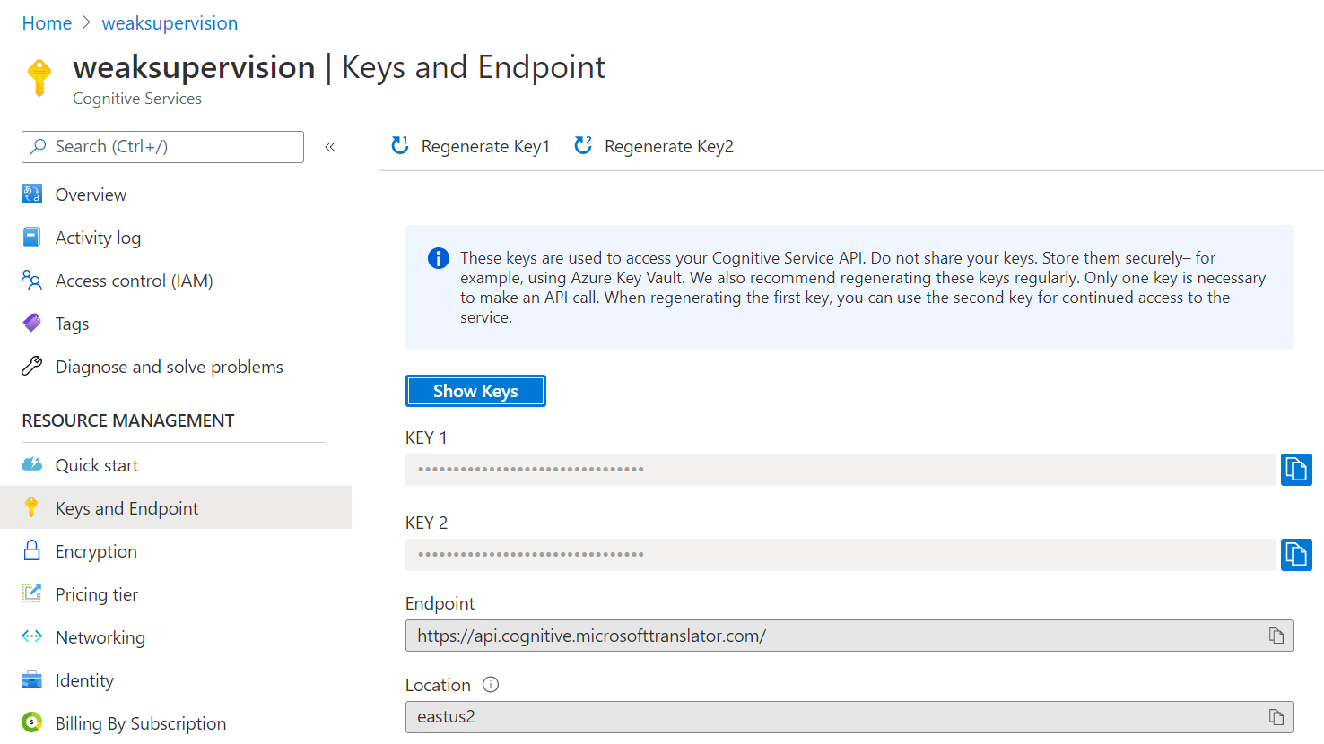
Figure 2-3. Azure Translator keys, endpoint, region
The transformation function request to translate the text is adapted from the GitHub Translator examples.
importos,requests,uuid,jsonimportspacynlp=spacy.load("en")resource_key="<RESOURCE_SUBSCRIPTION_KEY>"endpoint="<ENDPOINT>"region="<REGION>"deftranslate(text,language):headers={"Ocp-Apim-Subscription-Key":resource_key,"Ocp-Apim-Subscription-Region":region,"Content-type":"application/json","X-ClientTraceId":str(uuid.uuid4())}body=[{"text":text}]body=[{"text":text}]response=requests.post(endpoint+"/translate?api-version=3.0&to="+language,headers=headers,json=body)translation=response.json()[0]["translations"][0]["text"](translation)returntranslation@transformation_function()defaugment_by_translation(x):text=x["review_text"]french=translate(text,"fr")english=translate(french,"en")score=nlp(text).similarity(nlp(english))if(score<1.0):x["review_text"]=englishelse:x["review_text"]="DUPLICATE"returnx
The translate function takes the text to translate and the language as arguments, and returns the translated text. The augment_by_translation transformation_function invokes the translate function twice: to translate into French then back to English. The similarity of the original text and the translation is calculated through SpaCy’s similarity routine, which measures the cosine similarity between context-sensitive blocks of text (for the small models). Perfect duplicates would generate a score of 1.0.
Reusing the same example, the review for “Honest Illusions”, we can compare the initial English text, with the text obtained after re-translating the French output back to English.
English: “I simply adore this book and it’s what made me go out to buy every other Nora Roberts novel. It just amazes me the chemistry between Luke and Roxanne. Every time I read it I can’t get over the excitement and the smile it brings to me as they barb back and forth. It’s just an amazing story over the course of growing up together and how it all develops. Roxanne is smart and sassy and Luke is just too cool. This romantic duo shines and no one else compares to them yet for me. My very favorite romance.”
French: “J’adore ce livre et c’est ce qui m’a fait sortir pour acheter tous les autres romans de Nora Roberts. Ça m’étonne la chimie entre Luke et Roxanne. Chaque fois que je le lis, je ca obtenir sur l’excitation et le sourire qu’il m’apporte comme ils barbe et en avant. C’est une histoire incroyable au cours de sa croissance et comment tout se développe. Roxanne est intelligente et impersy et Luke est cool. Ce duo romantique brille et personne ne se compare à eux pour moi. Ma romance préférée.”
Back to English: “I love this book and that’s what made me come out to buy all the other novels of Nora Roberts. I’m surprised at the chemistry between Luke and Roxanne. Every time I read it, I can get on the excitement and smile it brings me as they beard and forward. It’s an incredible story during its growth and how everything develops. Roxanne is smart and impersy and Luke is cool. This romantic duo shines and no one compares to them for me. My favorite romance.”
Applying the transformation functions to the dataset
We now have the transformation functions. To be able to use them, we also need to decide upon a policy to use for applying each transformation function to the dataset in order to get a diverse, but realistic output. The Snorkel augmentation package contains several policies, for this purpose:
-
ApplyAllPolicy - This policy will take each data point, “book review” in our case, and apply all the transformation functions available to it, one by one, in the same order the
transformation_functionsare listed. The resulting text will be the product of having removed the adverbs, translated, and then supplied to gpt-2 for the next sentence prediction.
fromSnorkel.augmentationimport*tfs=[predict_next,augment_by_translation,spacy_remove_adverbs]policy=ApplyAllPolicy(len(tfs),n_per_original=1,keep_original=True)tf_applier=PandasTFApplier(tfs,policy)policy.generate_for_example()
The policy.generate_for_example object contains the list of the indices of the transformation functions selected to be applied to one particular data point, selected at random. The number of new data points to generate for each sample is defined by the n_per_original argument. For our case that would be all of them in order:
[[], [0, 1, 2]]
This policy will add one more data point per sample, doubling the dataset.
-
ApplyEachPolicy - unlike
ApplyAllPolicy, this policy will apply eachtransformation_functionto each data point, separately, without combining them.keep_originalindicates whether to keep the original data points in the augmented dataset.
policy=ApplyEachPolicy(len(tfs),keep_original=True)policy.generate_for_example()[[],[0],[1],[2]]
After applying this policy, for each data point, we will have 3 separate, new data points, each generated from one of the transformation functions.
-
ApplyOnePolicy - applies a single policy, the first one, to the data.
policy=ApplyOnePolicy(4,keep_original=True)policy.generate_for_example()[[],[0],[0],[0],[0]]
After applying this policy, for each dataset record, we will have an additional 4 records, generated using the first transformation functon from the list (the transformation function at index 0).
-
RandomPolicy - creates a list of
transformation_functionsby sampling the list oftfsat random. The length of this list is determined by thesequence_lengthargument.
policy=RandomPolicy(len(tfs),sequence_length=5,n_per_original=2,keep_original=True)policy.generate_for_example()[[],[1,2,1,2,2],[2,1,2,0,1]]
-
MeanFieldPolicy - this policy is probably the one that will have more uses because it allows the frequency of transformation function application to be defined by a user-supplied probability distribution. With this policy, a sequence of transformations will be applied to each data point, and the order/composition of that sequence will be determined by sampling from the list of transformation functions according to the supplied probability distribution.
policy=MeanFieldPolicy(len(tfs),sequence_length=1,n_per_original=1,keep_original=True,p=[0.3,0.3,0.4],)policy.generate_for_example()[[],[0]]
After selecting a policy, for our case we kept the MeanFieldPolicy we go ahead and apply the policy to the dataset and get the synthetic data points.
df_train_augmented=tf_applier.apply(df2)
A preview of some of the records of the augmented dataset is shown in table Table 2-15.
| review_text | reviewer |
|---|---|
I simply adore this book and it’s what made me… |
“Book Junkie” |
I love this book and that’s what made me come … |
“Book Junkie” |
I love this book and that’s what made me come … |
“Book Junkie” |
Magic, mystery, romance and burglary are all p… |
“Terry” |
Magic , mystery , romance and burglary are all… |
“Terry” |
Magic , mystery , romance and burglary are all… |
“Terry” |
I read the review and got the book and fell in… |
Diana |
I read the review and got the book and fell in… |
Diana |
I read the review and got the book and fell in… |
Diana |
It is difficult to find books in this genre th… |
A. Rowley |
It is difficult to find books in this genre th… |
A. Rowley |
It’s hard to find books like this that have a … |
A. Rowley |
This is one of my favorite Nora Roberts book. … |
avid reader “A reader” |
It’s one of my favorite Nora Roberts books. ."… |
avid reader “A reader” |
It ’s one of my favorite Nora Roberts books . … |
avid reader “A reader” |
This book has everything….Love, Greed, Murde… |
S. Williams |
This book has it all. One thing I really lik… |
S. Williams |
This book has everything. Some characters we… |
S. Williams |
When I began to read Nora Roberts, I really di… |
Creekergirl |
I began to read Nora Roberts , I did n’t expec… |
Creekergirl |
I began to read Nora Roberts , I did n’t expec… |
Creekergirl |
We can use this dataset now, to train supervised models.
Summary
Data Programming is a promising way to label data. The labeling functions or heuristics are learned on some sample data, and they are then applied to the entire dataset. A LabelModel is then trained over the weak labels generated and used to reconcile those weak labels into a final label. Snorkel has a good solution for data augmentation, as well, allowing practitioners to use several augmentations techniques at once, or select from a range of techniques controlling in what percentage each technique contributes to the added records.
In the next chapters, we will make use of Snorkel to practically label two datasets: one images and one text.
Bibliography
Alexander J. Ratner, Stephen H. Bach, Henry R. Ehrenberg, Chris Ré. Snorkel: Fast Training Set Generation for Information Extraction, 2017.
Benjamin Cohen-Wang, Alexander Ratner, Stephen Mussmann, Chris Ré. Interactive Programmatic Labeling for Weak Supervision, 2019.
Sonia Badene, Kate Thompson, Jean-Pierre Lorré, Nicholas Asher. Weak Supervision for Learning Discourse Structure, 2019.
Fred Sala, Paroma Varma, Chris Ré. Learning Dependency Structures in Weak Supervision, 2019.
Paroma Varma, Frederic Sala, Ann He, Alexander Ratner, Christopher Ré. Learning Dependency Structures for Weak Supervision Models, 2019.
Alexander Ratner, Braden Hancock, Jared Dunnmon, Frederic Sala, Shreyash Pandey, Christopher Ré. Training Complex Models with Multi-Task Weak Supervision, 2018.
Emmanouil A. Platanios, Hoifung Poon, Tom M. Mitchell, Eric Horvitz. Estimating Accuracy from Unlabeled Data A Probabilistic Logic Approach, 2017.
Jason Wei & Kai Zou. EDA: Easy Data Augmentation Techniques for Boosting Performance on Text Classification Tasks, 2019.
Alexander Ratner, Henry Ehrenberg, Zeshan Hussain, Jared Dunnmon & Christopher Ré. Learning to Compose Domain-Specific Transformations for Data Augmentation, 2017.
Adams Wei Yu, David Dohan, Minh-Thang Luong, Rui Zhao, Kai Chen, Mohammad Norouzi, and Quoc V.Le. Qanet: Combining local convolution with global self-attention for reading comprehension, 2018.
Sosuke Kobayashi. 2018. Contextual augmentation: Data augmentation by words with paradigmatic relations., 2018.
GPT-2 developers guide: https://github.com/openai/gpt-2/blob/master/DEVELOPERS.md
Amazon reviews dataset: https://nijianmo.github.io/amazon/index.html
Azure Translator https://azure.microsoft.com/en-us/services/cognitive-services/translator/
Vincent S. Chen, Sen Wu, Zhenzhen Weng, Alexander Ratner, Christopher Ré Slice-based Learning: A Programming Model for Residual Learning in Critical Data Slices, 2019.
Alexander J. Ratner, Henry R. Ehrenberg, Zeshan Hussain, Jared Dunnmon, Christopher Ré. Learning to Compose Domain-Specific Transformations for Data Augmentation, 2017.