![]()
Introduction to Statistical and Machine Learning Algorithms
This chapter will serve as a reference for some of the most commonly used algorithms in Microsoft Azure Machine Learning. We will provide a brief introduction to algorithms such as linear and logistic regression, k-means for clustering, decision trees, decision forests (random forests, boosted decision trees, and Gemini), neural networks, support vector machines, and Bayes point machines.
This chapter will provide a good foundation and reference material for some of the algorithms you will encounter in the rest of the book. We group these algorithms into the following categories:
- Regression
- Classification
- Clustering
Let’s first talk about the commonly used regression techniques in the Azure Machine Learning service. Regression techniques are used to predict response variables with numerical outcomes, such as predicting the miles per gallon of a car or predicting the temperature of a city. The input variables may be numeric or categorical. However, what is common with these algorithms is that the output (or response variable) is numeric. We’ll review some of the most commonly used regression techniques including linear regression, neural networks, decision trees, and boosted decision tree regression.
Linear Regression
Linear regression is one of the oldest prediction techniques in statistics. In fact, it traces its roots back to the work of Carl Friedrich Gauss in 1795. The goal of linear regression is to fit a linear model between the response and independent variables, and use it to predict the outcome given a set of observed independent variables. A simple linear regression model is a formula with the structure of
![]()
where
- Y is the response variable (i.e. the outcome you are trying to predict) such as miles per gallon.
- X1, X2, X3, etc. are the independent variables used to predict the outcome.
- β0 is a constant that is the intercept of the regression line.
- β1, β2, β3, etc. are the coefficients of the independent variables. These refer to the partial slopes of each variable.
- ε is the error or noise associated with the response variable that cannot be explained by the independent variables X1, X2, and X3.
A linear regression model has two components: a deterministic portion (i.e. β1X1 + β2X2 + ...) and a random portion (i.e. the error, ε). You can think of these two components as the signal and noise in the model.
If you only have one input variable, X, the regression model is the best line that fits the data. Figure 4-1 shows an example of a simple linear regression model that predicts a car’s miles per gallon from its horsepower. With two input variables, the linear regression is the best plane that fits a set of data points in a 3D space. The coefficients of the variables (i.e. β1, β2, β3, etc.) are the partial slopes of each variable. If you hold all other variables constant, then the outcome Y will increase by β1 when the variable X1 increases by 1. This is why economists typically use the phrase “ceteris paribus”“ or ”all other things being equal” to describe the effect of one independent variable on a given outcome.
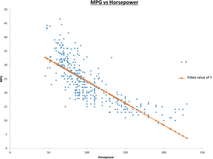
Figure 4-1. A simple linear regression model that predicts a car’s miles per gallon from its horsepower
Linear regression uses the least squares or gradient descent methods to find the best model coefficients for a given dataset. The least squares method achieves this by minimizing the sum of the squared error between the fitted and actual values of each observation in the training data. The gradient descent finds the optimal model coefficients by updating the coefficients in each iteration. The updates go in the direction so that the sum of errors between the model fitted and the actual values of the training data are reduced. Through several iterations it finds the local minimum by moving in the direction of the negative gradient, hence the name.
![]() Note You can learn more about linear regression from the book Business Analysis Using Regression: A Casebook (Foster, D. P., Stine, R.H., Waterman, R.P.; New York, USA; Springer-Verlag, 1998).
Note You can learn more about linear regression from the book Business Analysis Using Regression: A Casebook (Foster, D. P., Stine, R.H., Waterman, R.P.; New York, USA; Springer-Verlag, 1998).
Artificial neural networks are a set of algorithms that mimic the functioning of the brain. There are many different neural network algorithms, including backpropagation networks, Hopfield networks, Kohonen networks (also known as self-organizing maps), and adaptive resonance theory (or ART) networks. However, the most common is the back-propagation algorithm, also known as multilayered perceptron.
The back-propagation network has several neurons arranged in layers. The most commonly used architecture is the three-layered network shown in Figure 4-2. This architecture has one input, one hidden, and one output layer. However, you can also have two or more hidden layers. The number of input and output nodes are determined by the dataset. Basically, the number of input nodes equals the number of independent variables you want to use to predict the output. The number of output nodes is the same as the number of response variables. In contrast, the number of hidden nodes is more flexible.
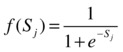
The development of neural network models is done in two steps: training and testing. During training, you show the neural network a set of examples from the training set. Each example has values of the independent as well as the response variables. During training, you show the examples several times to the neural network. At each iteration, the network predicts the response. In the forward propagation phase of training, each node in the hidden and output layers calculates a weighted sum of its inputs, and then uses this sum to compute its output through an activate function. The output of each neuron in the neural network usually uses the following sigmoidal activate function:
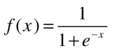
There are, however, other activation functions that can be used in neural networks, such as Gaussian, hyperbolic tangent (tanh), linear threshold, and even a simple linear function.
Let’s assume there are M input nodes. The connection weights between the input nodes and the first hidden layer are denoted by w1ij.
At each hidden node the weighted sum is given by
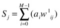
When the weighted sum is calculated, the sigmoidal activate function is calculated as follows:
After the activation level of the output node is calculated, the backward propagation step starts. In this phase, the algorithm calculates the error of its prediction based on the actual response value. Using the gradient descent method, it adjusts the weights of all connections in proportion the error. The weights are adjusted in a way that reduces the error the next time. After several iterations, the neural network converges to a solution.
During testing, you simply use the trained model to score records. For each record, the neural network predicts the value of the response for a given set of input variables (see Figure 4-2).
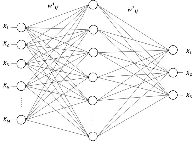
Figure 4-2. A neural network with three layers: one input, one hidden, and one output layer
The learning rate determines the rate of convergence to a solution. If the learning rate is too low, the algorithm will need more learning iterations (and hence more time) to converge to the minimum. In contrast, if the learning rate is too large, the algorithm bounces around and may never find the local minimum. Hence the neural net will be a poor predictor.
Another important parameter is the number of hidden nodes. The accuracy of the neural network may increase with the number of hidden nodes. However, this increases the processing time and can lead to over-fitting. In general, increasing the number of hidden nodes or hidden layers can easily lead to over-parameterization, which will increase the risk of over-fitting. One rule of thumb is to start with the number of hidden nodes equal roughly to the square root of the number of input nodes. Another general rule of thumb is that the number of neurons in the hidden layer should be between the size of the input layer and the size of the output layer. For example, (Number of input nodes + number of output nodes) x 2/3. These rules of thumb are merely starting points, intended to avoid over-fitting; the optimal number can only be found through experimentation and validation of performance on test data.
Decision Trees
Decision tree algorithms are hierarchical techniques that work by splitting the dataset iteratively based on certain statistical criteria. The goal of decision trees is to maximize the variance across different nodes in the tree, and minimize the variance within each node. Figure 4-3 shows a simple decision tree created with two splits of the data. The root node (Node 0) contains all the data in the dataset. The algorithm splits the data based on a defined statistic, creating three new nodes (Node 1, Node 2, and Node 3). Using the same statistic, it splits the data again at Node 1, creating two more leaf nodes (i.e. Nodes 4 and 5). The decision tree makes its prediction for each data row by traversing to the leaf nodes (i.e. one of the terminal nodes: Node 2, 3, 4, or 5).
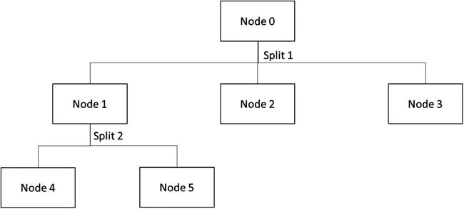
Figure 4-3. A simple decision tree with two data splits
Figure 4-4 shows a fictional example of a very simple decision tree that predicts whether a customer will buy a bike or not. In this example, the original dataset has 100 examples. The most predictive variable is age, so the decision first splits the data by age. Customers younger than 30 fall in the left branch while those aged 30 or above fall in the right branch. The next most important variable is gender, so in the next level the decision tree splits the data by gender. In the younger branch (i.e. for customer customers under 30), the decision tree splits the data into male and female branches. It also does the same for the older branch. Finally, Figure 4-4 shows the number of examples in each node and the probability to purchase. As a result, if you have a female customer aged 23, the tree predicts that she only has a 30% chance of buying the bike because she will end up in Node 3. A male customer aged 45 will have an 80% chance of buying a bike since he will end up in Node 6 in the tree.
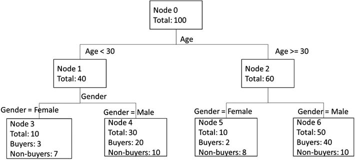
Figure 4-4. A simple decision tree to predict likelihood to buy bikes
Some of the most commonly used decision tree algorithms include Iterative Dichotomizer 3 (ID3), C4.5 and C5.0 (successors of ID3), Automatic Interaction Detection (AID), Chi Squared Automatic Interaction Detection (CHAID), and Classification and Regression Tree (CART). While very useful, the ID3, C4.5, C5.0, and CHAID algorithms are classification algorithms and are not useful for regression. As the name suggests, the CART algorithm can be used for either classification or regression.
How do you choose the variable to use for splitting data at each level? Each decision tree algorithm uses a different statistic to choose the best variable for splitting. ID3, C4.5, and C5.0 use information gain, while CART uses a metric called Gini impunity. Gini impunity measures the misclassification rate of a randomly chosen example.
![]() Note More information on decision trees is available in the book Data Mining and Market Intelligence for Optimal Market Returns by S. Chiu and D. Tavella (Oxford, UK, Butterworth-Heinemann, 2008) and at http://en.wikipedia.org/wiki/Decision_tree_learning.
Note More information on decision trees is available in the book Data Mining and Market Intelligence for Optimal Market Returns by S. Chiu and D. Tavella (Oxford, UK, Butterworth-Heinemann, 2008) and at http://en.wikipedia.org/wiki/Decision_tree_learning.
Boosted Decision Trees
Boosted decision trees are a form of ensemble models. Like other ensemble models, boosted decision trees use several decision trees to produce superior predictors. Each of the individual decision trees can be weak predictors. However, when combined they produce superior results.
As discussed in Chapter 1, there are three key steps to building an ensemble model: a) data selection, b) training classifiers, and c) combining classifiers.
The first step to build an ensemble model is data selection for the classifier models. When sampling the data, a key goal is to maximize diversity of the models, since this improves the accuracy of the solution. In general, the more diverse your models, the better the performance of your final classifier, and the smaller the variance of its predictions.
Step 2 of the process entails training several individual classifiers. But how do you assign the classifiers? Of the many available strategies, the two most popular are bagging and boosting. The bagging algorithm uses different random subsets of the data to train each model. The models can then be trained in parallel over their random subset of training data. In contrast, the boosting algorithm improves overall performance by sequentially training the models, testing the performance of each on the training data. The examples in the training set that were misclassified are given more importance in subsequent training. Thus, during training, each additional model focuses more on the misclassified data. The boosted decision tree algorithm uses the boosting strategy. In this case, every new decision tree is trained with emphasis on the misclassified cases to reduce the error rates. This is how a boosted decision tree produces superior results from weak decision trees.
It is important to watch two key parameters of the boosted decision tree: the number of leaves in each decision tree and the number of boosting iterations. The number of leaves in each tree determines the amount of interaction allowed between variables in the model. If this number is set to 2, then no interaction is allowed. If it is set to 3, the model can include effects of interaction of at most two variables. You need to try different values to find the one that works best for your dataset. It has been reported that 4-8 leaves per tree yields good results for most applications. In contrast, having only two leaves per tree leads to poor results. The second important parameter to tweak is the number of boosting iterations (i.e. the number of trees in the model). A very large number of trees reduces the errors, but easily leads to over-fitting. To avoid over-fitting, you need to find an optimal number of trees that minimizes the error on a validation dataset.
Finally, once you train all the classifiers, the final step is to combine their results to make a final prediction. There are several approaches to combining the outcomes, ranging from a simple majority to a weighted majority voting.
![]() Note You can learn more about boosted decision trees from the book Ensemble Machine Learning, methods and applications by C. Zhang and Y. Ma (New York, NY: pp. 1 - 34, Springer, 2012) and at http://en.wikipedia.org/wiki/Gradient_boosting#Gradient_tree_boosting.
Note You can learn more about boosted decision trees from the book Ensemble Machine Learning, methods and applications by C. Zhang and Y. Ma (New York, NY: pp. 1 - 34, Springer, 2012) and at http://en.wikipedia.org/wiki/Gradient_boosting#Gradient_tree_boosting.
Classification Algorithms
Classification is a type of supervised machine learning. In supervised learning, the goal is to infer a function using labeled training data. The function can then be used to determine the label for a new dataset (where the labels are unknown). A non-exhaustive list of classification algorithms that can be used for building the model includes decision trees, logistic regression, neural networks, support vector machines, naïve Bayes, and Bayes point machines.
Classification algorithms are used to predict the label for input data (where the label is unknown). Labels are also referred to as classes, groups, or target variables. For example, a telecommunication company wants to predict the following:
- Churn: Customers who have an inclination to switch to a different telecommunication provider
- Propensity to Buy: Customers willing to buy new products or services
- Up-selling: Customers willing to buy upgraded services or add-ons
To achieve this, the telecommunication company builds a classification model using training data (where the labels are known or have already been predefined). In this section, you’ll look at several common classification algorithms that can be used for building the model. Once the model has been built and validated using test data, data scientists at the telecommunication company can use the model to predict churn, propensity to buy, and up-selling labels for customers (where the labels are unknown). Consequently, the telecommunication company can use these predictions to design marketing strategies that can reduce the customer churn and offer services to the customers that are more willing to buy new services or up-sell.
Other scenarios where classification algorithms are commonly used include financial institutions, where models are used to determine whether a credit card transaction is a fraudulent case or if a loan application should be approved based on the financial profile of the customer. Hotels and airlines use models to determine whether a customer should be upgraded to a higher level of service (e.g. from economy to business class, from a normal room to a suite, etc.).
The classification problem is defined as follows: given an input sample of X = (x1, x2, ... xd), where xi refers to an item in the sample of size d. The goal of classification is to learn the mapping X → Y, where y Î Y is a class.
An instance of data belongs to one of J groups (or classes), such as C1, C2, ..., Cj. For example, in a two-class classification problem for the telecommunication scenario, Class C1 refers to customers that will churn and switch to a new telecommunication provider, and Class C2 refers to customers that will not churn.
To achieve this, labeled training data is first used to train a model using one of the classification algorithms. This is then validated by using test data to determine the number of mistakes made by the trained model (i.e. the classifier). Various metrics are used to measure the performance of the classifier. These include measuring the accuracy, precision, recall, and the area under curve (AUC) of the trained model.
In the earlier sections, you learned how decision trees, boosted decision trees and neural networks work. These algorithms are useful for both regression and classification. In this section, you will learn how support vector machines and Bayes point machines work.
Support vector machines (SVMs) were introduced by Bernhard E. Boser, Isabelle Guyon, and Vladimir N. Vapnik at the Conference on Learning Theory (COLOT) IN 1992. A SVM is based on techniques grounded in statistical learning theory, and is considered a type of kernel-based learning algorithm.
The core idea of SVMs is to find the separating hyperplane that separates the training data into two classes, with a gap (or margin) that is as wide as possible. When there are only two input variables, a straight line separates the data into two classes. In higher-dimensional space (i.e. more than two input variables), a hyperplane separates the training data into two classes. Figure 4-5 shows how a hyperplane separates the two classes, and the margin. The circled items are the support vectors because they define the optimal hyperplane, which provides the maximum margin.
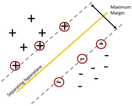
Figure 4-5. Support vector machine, separating hyperplane and margin
Consider the following example. Suppose a telecommunication company has the following training data consisting of n customers. Out of these n customers, let’s assume that 50 customers will churn, and the other 50 customers will not. For each customer, you extract 10 input variables (or features) that will be used to represent the customer. Given a customer who has used the service for some time, the data scientist and business analysts in the telecommunication company want to determine whether this customer will churn and move to a different telecommunication provider.
Suppose the training data consists of the following: (x1,y1), ... ,(xn,yn), where (xi,yj) denotes to xi mapped to the class yj. The hyperplane decision function is
![]()
where w and w0 are coefficients. A separating hyperplane will satisfy the following constraints:
![]()
![]()
An optimal separating hyperplane is one that enables the maximum margin between the two classes. These two constraints for describing the hyperplane can be represented using the equation
![]()
This equation can be used for representing all hyperplanes that can be used for separating the data. Often, the equation is not solved directly in its current form (also referred to as the primal form), due to the difficulty in directly computing the value of the norm of ||w||. In practice, the dual form of the equation is used for solving the optimization problem that will identify the optimal hyperplane.
![]() Note You can learn more about support vector machines and how the margin can be maximized from the following book:
Note You can learn more about support vector machines and how the margin can be maximized from the following book:
Vladimir, C. and Filip, M., Learning From Data (Concepts, Theory and Methods).
pp. 353 – 384 (Wiley-Interscience, 1998).
A good overview of support vector machines can be found at http://en.wikipedia.org/wiki/Support_vector_machine.
Azure Machine Learning provides a Two-Class Support Vector Machine module, which enables you to build a model that supports binary predictions. The inputs to the module can be either continuous and/or categorical variables. The module provides several parameters that can be used to fine-tune the behavior of the support vector machine algorithm. These include
- Number of iterations: Determines the speed of training the model. This parameter enables you to balance between training speed and model accuracy. The default value is set to 1.
- Lambda: Weight for L1 regularization used for tuning the complexity of the model that is produced. The default value of Lambda is set to 0.001. A non-zero value is used to avoid over-fitting the model.
- Normalize features: Determines whether the algorithm normalizes the values.
- Project to unit-sphere: Determines whether the algorithm projects the values to a unit-sphere.
- Random Number Seed: The seed value used for random number generation when computing the model.
- Allow unknown categorical levels: Determines whether the algorithm supports unknown categorical values. If this is set to True, the algorithm creates an additional level for each categorical column. The additional level is used for mapping levels in the test dataset that are not found in the training dataset.
Bayes point machines (BPMs) are a type of linear classification algorithm that was introduced by Ralf Herbrich, Thore Grapel, and Colin Campbell in 2001. The core idea of the Bayes point machine algorithm is to identify an “average” classifier that is able to effectively and efficiently approximate the theoretical optimal Bayesian average of several linear classifiers (based on their ability to generalize). The “average” classifier is known as the Bayes point. In empirical studies, Bayes point machines have consistently outperformed support vector machines for both lab and real-world data.
![]() Note The Bayes point machine algorithm used in Azure Machine Learning is based on Infer.Net and provides improvements to the original Bayes point machine algorithm. These improvements enable the Bayes point machine used in Azure Machine Learning to be more robust and less prone to over-fitting of the data. It also reduces the need to perform performance tunings.
Note The Bayes point machine algorithm used in Azure Machine Learning is based on Infer.Net and provides improvements to the original Bayes point machine algorithm. These improvements enable the Bayes point machine used in Azure Machine Learning to be more robust and less prone to over-fitting of the data. It also reduces the need to perform performance tunings.
Some of these improvements include the use of expectation propagation as the message-passing algorithm. In addition, the implementation does not require the use of parameter sweeping and having normalized data.
Recall the earlier definition of the classification problem: given an input sample X = (x1, x2, . . ., xd), where xi refer to an item in the sample of size d. The goal of classification is to learn the mapping X → Y, where y Î Y is a class.
Given an item in the sample xi, where xi is a vector with one or more variables. The BPM figures out the class label for xi by performing the following steps:
- Computing the inner product of xi with a weight vector w.
- Determining whether xi belongs to a class y, if (xi·w) is positive. (xi·w is the inner product of the vectors xi and w). Gaussian noise is added to the computation.
During training, the BPM algorithm learns the posterior distribution for w using a prior and the training data. The Gaussian noise used in the computation helps to address cases where there is no w that can perfectly classify the training data (i.e. when the two classes in the training data are not linearly separable).
![]() Note You can learn more about BPMs at http://research.microsoft.com/apps/pubs/default.aspx?id=65611.
Note You can learn more about BPMs at http://research.microsoft.com/apps/pubs/default.aspx?id=65611.
In addition, the following tutorial for using Infer.Net and BPMs provides insights into how the algorithm works:http://research.microsoft.com/en-us/um/cambridge/projects/infernet/docs/Bayes%20Point%20Machine%20tutorial.aspx.
Azure Machine Learning provides a Two-Class Bayes Point Machine module, which enables you to build a model that supports binary predictions. The module provides several parameters that can be used to fine-tune the behavior of the Bayes Point Machine module. These include
- Number of training iterations: Determines the number of iterations used by the message-passing algorithm in training. Generally, the expectation is that more iterations improve the accuracy of the predictions made by the model. The default number of training iterations is 30.
- Include bias: Determines whether a constant bias value is added to each training and prediction instance.
Similar to the Support Vector Machine Module, the parameter called Allow unknown categorical levels is supported.
Clustering Algorithms
Clustering is a type of unsupervised machine learning. In clustering, the goal is to group similar objects together. Most existing cluster algorithms can be categorized as follows:
- Partitioning: Divide a data set into k partitions of data. Each partition corresponds to a cluster.
- Hierarchical: Given a data set, hierarchical approaches start either bottom-up or top-down when constructing the clusters. In the bottom-up approach (also known as agglomerative approach), the algorithm starts with each item in the data set assigned to one cluster. As the algorithm moves up the hierarchy, it merges the individual clusters (that are similar) into bigger clusters. This continues until all the clusters have been merged into one (root of the hierarchy). In the top-down approach (also known as divisive approach), the algorithm starts with all the items in one cluster, and in each iteration, divides into smaller clusters.
- Density: Density-based algorithms grow clusters by considering the density (number of items) in the “neighborhood” of each item. They are often used for identifying clusters that have “arbitrary” shapes. In contrast, most partitioning-based algorithms rely on the use of a distance measure. This produces clusters that have regular shapes (e.g. spherical).
![]() Note Read a good overview of various clustering algorithms at http://en.wikipedia.org/wiki/Cluster_analysis.
Note Read a good overview of various clustering algorithms at http://en.wikipedia.org/wiki/Cluster_analysis.
In this chapter, we will focus on partitioning-based clustering algorithms. Specifically, you will learn how k-means clustering works.
For partitioning-based cluster algorithms, it is important to be able to measure the distance (or similarity) between points and vectors. Various distance measures include Euclidean, Cosine, Manhattan (also known as City-block) distance, Chebychev, Minkowski, and Mahalanobis distance.
In Azure Machine Learning, the K-Means Clustering module supports Euclidean and Cosine distance measures. Given two points, p1 and p2, the Euclidean distance between p1 and p2 is the length of the line segment that connects the two points. The Euclidean distance can also be used to measure the distance between two vectors. Given two vectors, v1 and v2, the Cosine distance is the cosine of the angle between v1 and v2.
The distance measure used for clustering is chosen based on the type of data being clustered. Euclidean distance is sensitive to the scale/magnitude of the vectors that are compared. For example, even though two vectors seem relatively similar, the scale of the features can affect the value of the Euclidean distance. In this case, the Cosine distance measure is more appropriate, as it is less susceptible to scale. The cosine angle between the two vectors would have been small.
K-means clustering works as follows:
- Randomly choose k items from the data set as the initial center for k clusters.
- For each of the remaining items, assign each one of them to the k clusters based on the distance between the item and the cluster centers.
- Compute the new center for each of the clusters.
- Keep repeating step 2 and 3 until there are no more changes to the clusters, or when the maximum number of iterations is reached.
To illustrate, Figure 4-6 presents a data set for k-means clustering. There are three distinct clusters in this data, which are illustrated with different colors.
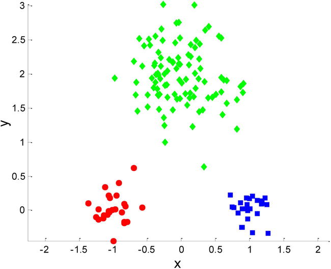
Figure 4-6. Data set for k-means clustering
Figure 4-7 illustrates k-means clustering with k=3 and how the three cluster centroids, represented as + symbols, move each iteration to reduce the mean squared error and more accurately reflect the cluster centers.
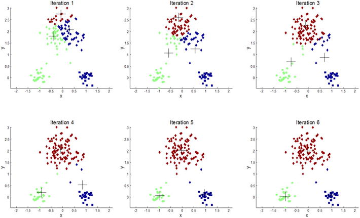
Figure 4-7. Iterations of the K-means clustering algorithm with k=3 in which the cluster centroids are moving to minimize error
The K-Means Clustering module in Azure Machine Learning supports different centroid initialization algorithms. This is specified by the Initialization property. Five centroid initialization algorithms are supported. Table 4-1 shows the different centroid initialization methods supported.
Table 4-1. K-Means Cluster - Centroid Initialization Algorithms
|
Centroid Initialization Algorithm |
Description |
|---|---|
|
Default |
Picks first N points as initial centroids |
|
Random |
Picks initial centroids randomly |
|
K-Means++ |
K-Means++ centroid initialization |
|
K-Means+ Fast |
K-Means++ centroid initialization with P:=1 (where the farthest centroid is picked in each iteration of the algorithm) |
|
Evenly |
Picks N points evenly as initial centroids |
Summary
In this chapter, you learned about different regression, classification, and clustering algorithms. You learned how each of the algorithms work, and the type of problems for which they are suited. The goal of this chapter is to provide you with the foundation for using these algorithms to solve the various problems covered in the upcoming book chapters. In addition, the resources provided in this chapter will help you learn more deeply about the state-of-art in machine learning, and the theory behind some of these algorithms.