7.1.1 Composing the Risk Model Structure

As a first step in your risk model implementation you will need to determine how to aggregate the exposures from different business activities in a hierarchy that ultimately combines all exposures into one total exposure. Grouping your exposures from the bottom up will allow you to reflect organisational accountability and limits for risk from traders and desks up to the level of the entire organisation.

Trader positions are rolled up into desk-level positions, which in turn are then rolled up by product group or division and so on until you finally arrive at the organisation level.

7.1.1.1 Basic Exposures at Trader or Desk Level

Figure 7.2 shows the roll up of individual exposures from trader/desk level portfolios at the bottom, each with the individual holdings up to the level of the total organisation. In the example, the trader/desk level portfolios are split by product type. Each trader/desk thus has a trading portfolio that contains only products of a specific type like equities, fixed income securities, loans, and the like.

Figure 7.2: Example risk exposure aggregation hierarchy with three layers.

For example, the trader/desk portfolio SECURITIES-Equity should only contain positions in equity instruments.

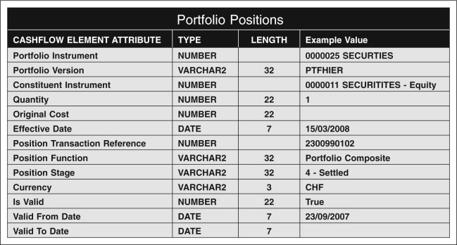
In Figure 7.3 you can see the trader/desk portfolio SECURITIES-Equity expanded to show the holdings in the portfolio in form of a tree diagram. Each leaf in the tree in Figure 7.3 will need to be represented by a position record in the database using the record structure set out in Figure 7.4.

Figure 7.3: Position exposures in a trading portfolio.

Figure 7.4: Structure for position records for base level and aggregate positions.

In Figure 7.5 you can see an actual example for a trading position in the ordinary shares of Microsoft Inc. in the trader/desk portfolio SECURITIES-Equity.

Figure 7.5: An example of position record for a base level trading position.

Detailed positions from this level give the actual exposures to individual instruments. In Figure 7.6 you can see how the same record can be used to record the Mark-to-Market Profit or Loss over a given holding period for the position from Figure 7.5.

Figure 7.6: Profit/loss for a given trader/desk level trading position.

7.1.1.2 Aggregate Exposures

To analyse risk across your business you will need to aggregate exposures all the way up to the level where you have a total aggregated portfolio covering your entire business as shown in Figure 7.2.

You can build up aggregate exposures using the same machinery as that which you use to record and track exposures at the trader or desk level. Each aggregate portfolio is there again set up as a portfolio instrument itself.

The aggregate portfolio SECURITIES in Figure 7.7 can thus be defined as a portfolio instrument and the trader/desk level portfolios SECURITIES–Equity and SECURITIES–Fixed-Income can be linked to the composite via a special running position record for each.

Figure 7.7: Aggregation of exposures to higher levels.

The example running position record linking the base portfolio SECURITIES–Equity to the Composite portfolio SECURITIES can be seen in Figure 7.8.

Figure 7.8: Aggregating exposures to the level covering the entire business.

Analogously, the Global Composite Portfolio in Figure 9.10 (of Chapter 9) can yet again be built the same way as the composite portfolio EUROPE. The All Business aggregate exposure portfolio should thus be set up as a portfolio instrument. Then each of the component aggregates, SECURITIES, CREDIT, and DERIVATIVES can be linked to it using a portfolio position record similar to the one in Figure 7.9.

Figure 7.9: Position record linking lower level exposures to a higher aggregate level.

Once the exposure aggregation hierarchy is completely set up it is possible to create detailed roll-up exposures for each instrument from individual trader/desk level positions to instrument-by-instrument aggregate positions at the firm level.

These positions from trader/desk level upward give you the instrument exposures you will need to calculate VAR or ETL for any given portfolio at any level in the hierarchy.

7.1.2 Mapping Building Blocks to Risk Models

The second main step in a risk model implementation is to map the information in your instrument database to your risk models. Mappings in risk models are similar to or extend those you have already created for instrument pricing models.

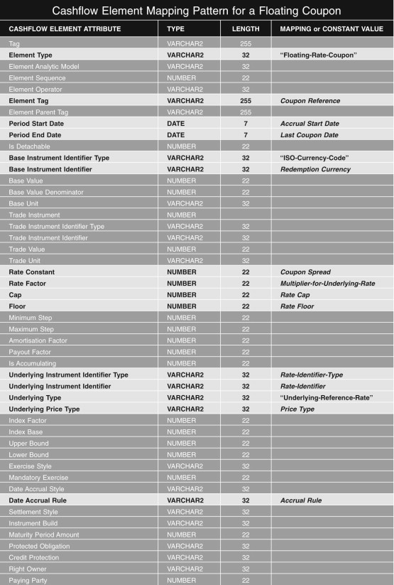
In Figure 7.10 you can see a mapping that shows how to obtain the parameters for a Parametric VAR/ETL model from the terms of an Equity Call Option building block such as the one given in Figure 7.13. Some parameters such as the Strike Price can be read directly from the terms of the Equity Call Option building block whereas others such as the Volatility of the Underlying or the current Spot Price can be looked up in other parts of the database with the help of the terms of the Equity Call Option building block. In Figure 7.11 and 7.12 you can see the description of a bullet redemption and floating rate coupon feature respectively which together would define the key parts of the financial characteristics of a floating rate bond as needed as input for a risk model.

Figure 7.10: Mapping an equity call option to the Black & Scholes option pricing model.

Figure 7.13: Mapping an equity option to the cash flow element structure.

Figure 7.11: Mapping a bullet redemption to the cash flow element.

Figure 7.12: Mapping a floating rate coupon to the cash flow element structure.

A few remaining ones like the riskless interest rate and the valuation date need to be set up when the model is configured for a particular purpose or given to the model when it is actually run.

We recommend to deepen your intuition about risk model mapping using Lab Exercise 7.1.

7.1.3 Creating and Calibrating Risk Model Inputs

Many model inputs, like the coupon rate of a fixed coupon bond or the strike price of an option, are static reference data and can be obtained from the terms of instrument building blocks like coupons, redemptions and options. Nevertheless, all risk models also need further inputs related either to the instrument itself, its issuer, or the market more generally. Figure 7.14 illustrates how the model calibration process derives calibration parameters for risk modeling using reference and market.

Figure 7.14: Model calibration and pre-processing input data.

Among the most important of these inputs is the Variance-Covariance matrix, which is critical for both Parametric VAR/ETL as well as Monte Carlo based VAR/ETL. Others include the yield curves for risk free and risky interest rates, or the Beta for a given firm or equity instrument, or the volatility of a share used as underlying in an equity option.

It makes sense to distinguish those into two categories:

• 1. the calculation of constructs like yield curves, which can be called model calibration (or just calibration) since a yield curve and similar constructs provide generic parameters for models not directly related to an instrument to be valued.
• 2. the task of pre-processing input data such as a time series of market prices of an instrument, some index or time series for related dividends or earnings, and other data into a forecast for the price volatility of the instrument, its Beta relative to the benchmark, the growth rate of the dividend or earnings stream over time.

In some cases this pre-processing can be fully automated, but in others it will involve considerable human input and intervention. Measuring the historical Beta or Volatility can be fully automated. Volatility and Beta forecasts can sometimes be automated but at least need to be monitored closely. Others like earning or even dividend forecasts usually need substantial input and intervention from analysts.

In your implementation you need to determine which types of calibration and pre-processed inputs you need. Then you need to determine how they can best be mapped into your modelling database. After that you need to decide which type of process will create the calibration and pre-processed inputs, whether this process is part of your implementation, or external to it. If the process is external to your implementation you need to decide how you can best feed them into your database, and whether these feeds can be fully or partly automated. You can use Figure 7.15 as starting point for a checklist to guide you through the process of deciding what calibration processes you may need and how to realize them.

Figure 7.15: Checklist for implementing calibration and pre-processed input data.

If any calibration and pre-processed input data is part of your project and cannot be obtained from another source, you will then need to decide if their creation can be fully or partially automated. Otherwise, it remains a manual activity for the user of your pricing models. If any can be automated you will need to ensure that they fit into your overall processes. Where necessary, they need to be supported by tools such as input (or operator) screens, parameter files so that your users or model operators can adjust the processes to changing circumstances.

7.1.4 Creating Risk Measurement Processes

Once your reference and market data is in your database, and you have correctly set up your exposure aggregation hierarchy, mapped all building blocks to pricing models and implemented those risk analysis models, and completed any work for automating feeds or the creation of calibration and preproceessed input data, you will still need to orchestrate the overall risk measurement calculation process.

The end-to-end process usually comprises many subprocesses, all of which need to be coordinated. Figure 7.16 illustrates a typical end-to-end process in three stages. Although it is possible to do this coordination across subprocesses manually, more often than not this would be very risky and costly in terms of required manpower. If this is the case you need to decide how you can implement the orchestration for your valuation solution with the resources you have at hand. In some cases it is possible to write a simple program component or even just a script that ties all your processes together.

Figure 7.16: End-to-end risk measurement process.

Usually, however, you need a more flexible solution than that. One of the big benefits of the building block approach is its flexibility and the ease and speed with which you can adapt to new financial products or new approaches to pricing particular atomic building blocks. This benefit would be lost if you implement your solution as one monolithic block so that your whole solution has to be reworked, retested, and reinstalled every time you want to change your high-level end-to-end process that runs your valuation models or any time you want to add or modify a single building block valuation model.

One way to avoid this predicament is to use a meta model for defining your high-level end-to-end process and then either create some software yourself that lets you execute the process as defined by the meta model or to use a readymade solution to both define and run your process.

Before you jump into building such a solution yourself make sure you are both an expert in executable process models, the implementation of process schedulers, and a glutton for extreme punishment. The smarter way to implement your end-to-end process is to use a commercial ready-to-use solution for this. The easiest, quickest, and often the most robust solution specifically designed for the implementation of end-to-end pricing are risk and performance measurement processes such as Fincore Financial’s Analytics Hub (www.fincorefinacial.com).

Alternatively you could use a generic solution such as the ORACLE business process orchestration toolkit, or you could use a process scheduler your organisation already uses together with any middleware you may need to link up your models, the scheduler, and your database. Although it is not as bad as building your own from scratch, this alternative still involves a substantial amount of effort, risk, and costs, and you should think very carefully whether using a generic process orchestration toolkit or an existing general purpose scheduler and some glue logic will be meeting your needs.

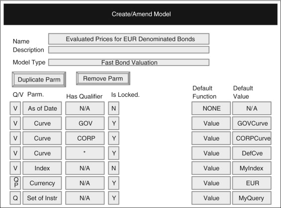
If you use a solution specifically designed for the implementation of end-to-end risk measurement processes such as Fincore Financial’s Analytics Hub, you will be able to focus on designing your models and process, and will not have to spend time creating the infrastructure they need to operate. Figures 7.17 and 7.18 illustrate how easy it can be to set up your end-to-end process. Figure 7.18 shows how you could register an existing or new pricing model and set up its parameters.

Figure 7.17: A meta model for your high level valuations process.

Figure 7.18: Registering valuation model components as part of a process meta model.

Such parameters can be either values or queries you can enter and save in a different screen that select the data according to your given criteria when the end-to-end process is run. Such user-defined queries give you full control over the process and are very powerful. A single risk model could be set up many times, each time with different parameters. Each such model configuration thus would operate on different instruments and with different calibrations or different versions of input data.

Figure 7.19 shows how you might put together different models into one overall process simply by choosing from your pool of model configurations.

Figure 7.19: Creating a process template ready to be run using a process scheduler.

7.1.5 Refining Your Risk Model Implementation

Risk Model implementation involves large numbers of assumptions and judgement calls that have to be made well before a result becomes visible. It is inevitable that at least some assumptions and judgement calls will have to be revised.

The fewer assumptions and judgement calls are involved and the quicker you can get to the point where you can check them against real results, the easier it will be to identify what needs to be changed and to put the revisions into practice.

In Chapter 1 we introduced the fountain model for model implementation that is reproduced in Figure 7.20. It provides a robust framework that will help you make sure that frequent small iterations do not veer off course and your implementation becomes an exercise in “extreme model hacking.”

Figure 7.20: Iterative refinement of model implementations.

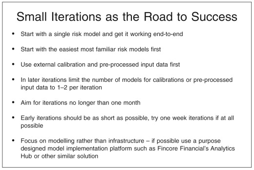
In practical terms this means that you should start your implementation with one or at most two risk models that are easiest and with which you have most experience. If these models can be mapped to many atomic building blocks, start by covering at most a handful of atomic building blocks from those that can be mapped to the models you are actually implementing. Even for simple historical data-based risk models this will still leave you with a challenging amount of effort. Figure 7.21 gives you a checklist to use as a starting point for keeping your iterations small, manageable, and productive.

Figure 7.21: Small iterations as the road to success.

7.2.1 Methodology Perspective: Risk Governance Oversight

In this perspective you take a town planner’s view of your risk implementation. What is important is that you make the ground rules to fit the size and nature of your endeavour. If you simply tinker with risk models on the side, perhaps to explore their potential or better understand them, then you will need very little groundwork in this perspective.

If, on the other hand, your risk models are used for key financial decision making or will be used as part of a service or product then the work that has to be undertaken in this perspective will be substantial. The key points your planning should cover are:

• Who will use your risk models and for what purpose will they be used?
• What will happen if your risk models are wrong or unavailable?
• Who would have to answer the questions if things go wrong after this or the next few iterations: you or your team, your boss, the CEO or the Chairman of the Board of your organisation?
• Have you included the right people in the dialogues or workshops for setting out the ground rules?
• Have you done enough work to make the ground rules robust enough for the current stage?
• Have you we covered all the different dimensions from Goals to Process?
• Are the ground rules just right: easy to understand, easy to put into action, easy to measure but complete, consistent, and comprehensive enough to rule out pitfalls into which you or your team, your division, or even your whole firm might fall?

7.2.2 Business Perspective: Risk Business Ownership

In this perspective you take the view of a business owner. Two questions are always (or at least always should be) on a business owner’s mind:

• How will this make us more profitable?
• How will this protect your business from failing?

Thus you will need to probe for how your risk measures and the way you create them add value to your business, to that of your sponsors or that of your clients. Yet again, check how your risk models—when they go wrong—could endanger your business or that of your sponsors or clients. The key points your planning should cover are:

• Are the risk models and process for creating them fit for the intended purpose?
• Does your proposed way of creating risk models fully exploit the potential for adding value to your business or that of our sponsors or clients?
• Can you do this more cheaply, faster, with less resources, fewer errors, or in a more informative way?
• What is the biggest hole you can fall into with the chosen approach to risk modelling and how would you get out of it? Would you survive the fall?
• Have you got the resources to see our plan through to completion? Can you see it through beyond completion and all the way until it will be a success?

7.2.3 Architecture Perspective: Risk Model Designer

The designer’s—or architect’s—perspective is dealing the decisions that set the framework for how your models will be implemented in detail. Some of these decisions may be given quantities if you already have a technical infrastructure for your implementation that you must use.

The challenge for the designer is to shape the remaining points in the framework in such a way that both the model builder’s work and the model operator’s efforts will together yield the desired results both now and in the distant future. The key points your planning should cover are:

• What is the right infrastructure for your implementation?
• Do you have the right infrastructure, and if not, how can you get it?
• Will your proposed implementation work with your given data feeds and the skills and experience of the people who will operate the models?
• What is the road map that will deliver as much value as possible as early as possible?
• Are you using this roadmap? If not, what stops you from using it and how can you remove and such blocks?

7.2.4 Systems Perspective: Risk Model Builder

The system builder’s perspective deals with the shop floor decision of how to actually code and put together the risk model solution. Here, you can rely on a lot of ground work already laid by the other perspectives. The bigger picture in terms of what you aim to achieve, the pitfalls to avoid, and the constraints given or agreed should already be clear. Thus, you can now focus on the details of the implementation. The key points your planning should cover are:

• Are you implementing the model in the best way possible?
• Are there faster or more predictable ways at arriving at the same result?
• Are you handling all the pitfalls that your valuation model may face?
• Can and do you double-check the results? If not is this OK under the circumstances? If the answer is yes, would your boss, the CEO or your clients or regulators agree? If they would agree now would they still agree if our risk measurements went horribly wrong and undetected for some time?
• If you detect a problem later or a better method becomes available, how difficult would it be to switch? If it is difficult, what can you do now to make that switch easier?

7.2.5 Operating Perspective: Risk Model Operator

The operator’s perspective is dealing with what it is like to use the risk measurement solution to produce actual VAR or ETL measures under actual operating conditions rather than what may have been assumed or planned. The key points your planning should cover are:

• Do you fully understand the capabilities and limitations of the solution? If not, where do you lack information and how could you bridge this gap?
• Can you run the solution in such a way as to produce valuations to an agreed standard with the given data feeds and the given expertise of the team?
• If not what are the problems and what can be done in the short term to overcome them?
• How can you help the implementation team to overcome these challenges in the medium to long term?
• Are you making the best use of the solution? If not what would you need to do to get there?
• What could go wrong with the way you operate the solution? What is the impact on the business and our clients in the worst case? Are there ways of mitigating this? Are there ways in which the solution could be operated differently that would result in a more favourable worst case or at least reduce the impact?