Pins

“Pins” is a generic term for things that, historically, looked like pins but these days, often do not. For the purposes of this book, a pin is a conductive area connected to the microcontroller through which communication may take place with external peripherals. Figure 9-1 shows a close-up picture of the “pins” on the micro:bit:

Figure 9-1. Pins on a micro:bit

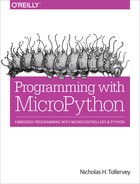
They don’t look like pins at all, and some of them are big enough for you to attach an alligator clip. The pins form the bottom edge of the board, and you may be wondering how you are supposed to connect things to all the smaller pins. The answer is to use an edge connector into which you plug jumper cables connected to external peripherals or a breadboard onto which you can place external components (Figure 9-2).

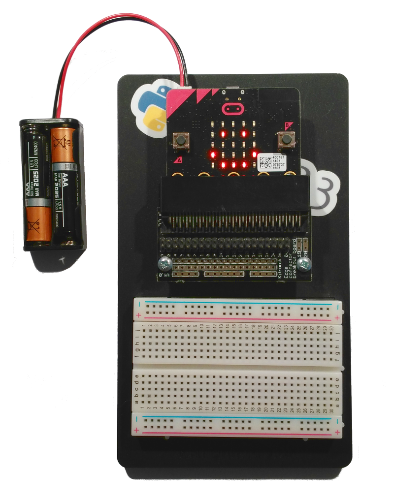
Figure 9-2. A micro:bit in an edge connector attached with an adjacent breadboard

The pins on a Circuit Playground Express are all like the micro:bit’s—large for alligator-clip-related reasons. In contrast, the PyBoard comes in two configurations: without any pin connections (there are just holes in the circuit board into which one solders such connectors) or pre-soldered with female pins into which one pokes jump cables to which you attach the external peripherals. The ESP8266/32-based boards often come with male pins pre-soldered onto the board—at last, devices with GPIO pins that actually look like pins!

Pins are named so we can reference them in our code. References to pins are found in different places, depending on the version of MicroPython you have running on your device. If you’re using the micro:bit you’ll find them in the microbit module. They’re in the board module if you’re using CircuitPython with Adafruit devices. Both the original PyBoard and the ESP8266/32 ports of MicroPython have a Pin class that you instantiate with the name of the pin and some notion of its characteristics (for example, that it’s a digital input).

Names are usually printed onto the board so it is possible to look at the pin and work out what it’s called. Different pins may be used for difference sorts of things. Some pins simply provide electrical current at an advertised voltage in order to power an external peripheral. The “3v” pin on the micro:bit is a good example of this sort of pin, and you can think of it as the equivalent of the positive end of a battery.

Other pins act as ground (often labelled GND), which is the equivalent of the negative end of a battery. The pins that only provide current and those labelled ground are not under your control since they only do what their name suggests.

It is the other pins that are more interesting to us and they may be capable of doing different sorts of things. For instance, all of them will be capable of acting as digital pins. You control them to be either low (0 V) or high (producing current at the board’s supply voltage, often 3.3 V). Some others will be able to act as analog pins, capable of sending or receiving signals that are not high or low but may be somewhere between each extreme. Usually such graduation in value is manifested as differences in voltage that are read by an analog-to-digital converter (ADC) and turned into a number within a certain range. Analog output is created by a digital-to-analog converter (DAC) that takes a number and turns it into a voltage representation of the analog value. Of course, digital pins can pretend to be analog by using the pulse width modulation trick described Chapter 7. Finally, some pins are configured in such a way as to allow them to respond to capacative touch (as described in Chapter 8).

Remember that GPIO pins can be in three default input states: high, low, and floating. By setting the “pull” of the pin (to high or low), we avoid the indeterminate floating state whose signal will reflect the ambient electrical conditions of the pin.

On some boards, it is possible to define interrupts that kick in if their input changes. This generally follows the pattern of defining a simple callback function to handle the interrupt and assigning it to a type of change on a specific pin. The following example for the ESP8266 boards demonstrates this:

from machine import Pin

def callback(p):
    print('Pin', p)

p0 = Pin(0, Pin.IN)
p0.irq(trigger=Pin.IRQ_FALLING, handler=callback)

The callback function receives an object representing the pin, p, that triggered the interrupt and prints it. Such hard interrupts trigger as soon as the expected event occurs, interrupting any running code. As a result, the callback functions that handle such interrupts are limited in what they can do (for example, they cannot allocate memory) and should be as simple as possible.

Next, an input pin is defined, and we assign the callback function as a handler for an interrupt request (IRQ) by defining the trigger (the pin drops from a high to low state) and referencing the callback function. From this moment on, if you apply high and then low voltages to pin 0, you’ll see the results of the print function used in the callback.

Sometimes you only need to use a single pin to send or receive a signal. This is called serial communication, since the data is sent sequentially, a single bit at a time. Alternatively, you may need to send or receive data via multiple pins. This is called parallel communication, as several bits are sent at once over the available channels of communication. Such connections that carry signals between devices and components are called a bus.

To work out what pins work in what way (if the name of the pin doesn’t tell you that already), you should consult the pinout diagram for the device. Figure 9-3 shows what the micro:bit’s pinout looks like.

Notice how each pin has a name and some indication of its function. Some of the pins are re-used to control things like the LEDs on the display. Rather than reproduce pinouts in this book (that with new iterations of boards may result in changes), I suggest you look online for them, typing the name of the device and the word “pinout” into a search engine.

While this sort of information is useful, many of the peripherals you will want to use with your boards use protocols that sit on top of the physical capabilities of the various GPIO pins. It is to three of these protocols that we turn our attention for the rest of the chapter. Once you understand the basics of each of these protocols, it should be a relatively simple task to connect a peripheral, read its associated data sheet (produced by the manufacturer), and work out how to use the expected protocol to make use of it.

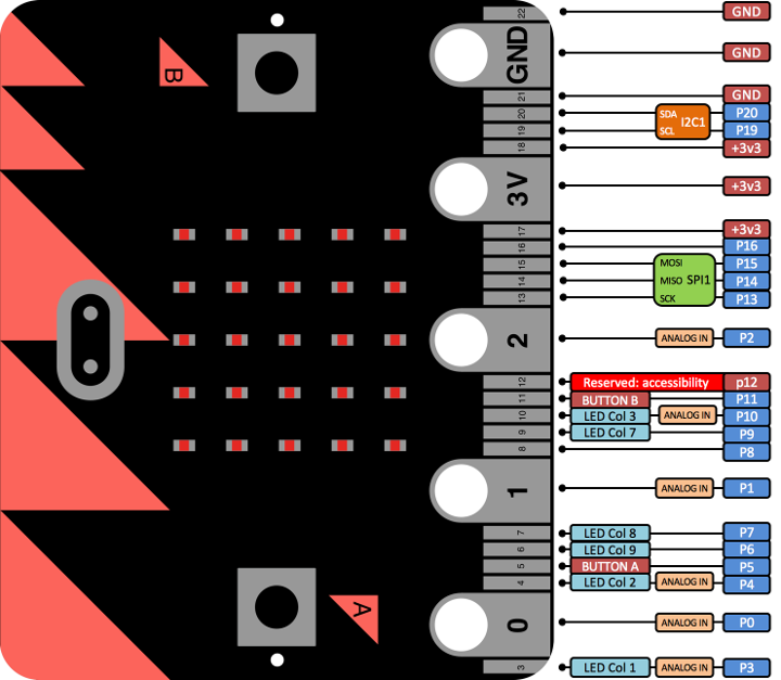
Figure 9-3. The micro:bit’s pinout diagram

UART

When you plug a board into your computer via the USB cable it is possible to communicate with the device using the REPL. What makes that possible is the universal asynchronous receiver/transmitter (UART), a part of the microcontroller that mediates between serial and parallel communication. Serial messages come in one bit at a time (a high/low signal), and the UART hardware assembles the signal into bytes (a parallel representation usually consisting of 8 bits) that are sent via an internal bus for further processing by the microprocessor. Conversely, to send a message the UART takes a byte and turns it into a series of high/low signals representing the constituent bits.

For this to work, several arrangements need to be made. First, the transmitting port (usually called TX) of device A must connect to the receiving port (usually called RX) of device B, and vice versa.

Second, there also needs to be agreement about the timing of the serial communication so the UART can detect the individual high/low signals. This is the speed of communication and is expressed as one of several standard baud rates: 9600, 14400, 19200, 28800, 38400, 57600, and 115200 bits per second.

Third, sometimes you may need to specify the number of bits per byte (although the standard is usually 8). You may also need to specify whether to use a parity bit (whose function is to detect errors in transmission), and the number of stop bits that signal the end of a unit of transmission.

The UART also has a “"first in/first out” (FIFO) queue so bytes can be buffered if they are not read as soon as they’re received.

By default, the UART on MicroPython boards is connected to the internal USB-UART TX/RX pins that connect to a USB serial convertor, thus connecting the UART to your PC via the USB port. On the PC end of things, a library like pySerial or a tool like picocom opens a serial connection via a USB port on your PC, thus enabling you to send and receive data to and from the Python REPL. The default baud rate for connecting to MicroPython in this way is 115200.

UART interactions in MicroPython require that the connection is configured (specifying the pins, baud rate, and other attributes already discussed). Each board has a slightly different way to instantiate and configure the UART although, at a conceptual level, they all work in the same way. Once configured, you will be working with a byte stream with familiar methods such as read, readline, and write. This is consistent across all platforms. The following micro:bit-based example is typical and demonstrates how to use the UART to read and write to a connected PC via the USB-serial bus:

from microbit import *

while True:
    msg = uart.read()
    if msg:
        uart.write(msg)

This short script simply echos anything it receives (it uses the default UART settings, so it is receiving and transmitting via the USB port). If you connect to the device in the same way you would with the REPL, it will just reply with any of the characters you type. It’s a very basic example, but all the fundamentals are contained within the script: read from the buffer and write a response. It is important to note that the micro:bit has a uart object that mediates such communication. Other boards will require you to instantiate a UART class with the right configuration for your needs. In this case, please consult the documentation for the port of MicroPython that targets your device. It’s also important to point out that UART isn’t just for REPL- or USB-based interactions; it can be used to facilitate all sorts of useful yet simple inter-device communication.

SPI

As the name suggests, the serial peripheral interface (SPI) is another serial protocol whose aim is to facilitate communication with peripherals. However, it is different from using the UART in a number of important ways.

As you know, the UART is an asynchronous protocol, meaning there is no signal used to indicate timing synchronisation to an agreed single clock when communicating between devices. All each device knows is the expected baud rate (speed) of transmission that has been agreed in advance. However, this can be a problem if the two devices have slightly different clocks: if the receiver samples the signal at the wrong time (to ascertain the high or low state on the pin), it will end up producing garbage. To work around this problem, the transmitting UART will add bits (for example, the stop bit) to help the receiving UART synchronise with the data as it arrives. Differences in data rate are not usually a problem in this case because the receiver will re-synchronise upon receipt of the stop bit. However, such asynchronous communication adds a lot of overhead in the form of stop bits, and the relatively complicated UART hardware needed to make such communication possible. Sometimes we need to connect with relatively simple peripherals that may not have such capabilities built in.

SPI takes a different approach: it’s a synchonous data bus, and there is a notion of hierarchy of devices.

SPI is synchronous because one of the connections between devices is an oscillating clock signal that tells devices exactly when to sample the high or low states of the signal (usually labelled as SCLK). As a result, the measures and complexity introduced to mitigate differences in clocks in UART-based communication are replaced by the clock signal.

You may wonder how devices tell where the clock signal comes from. This is answered by the hierarchical nature of SPI.

There is a primary device (usually the microcontroller) that, by prearrangement, supplies the clock signal. By convention, this is called the master with any other device connected via SPI referred to as slave[s].¹ In a similar way to how UART has TX and RX connections, the SPI protocol calls its data transmission connections MOSI (master out, slave in) and MISO (master in, slave out). All the slave devices receive and transmit on the same MOSI and MISO connections, so there needs to be some way to differentiate between signals to and from specific slave devices. This is achieved by the chip select (CS) connection (also sometimes called slave select). This connection indicates when a slave device should send and/or receive data and is done in an active-low configuration: the pins are pulled high by default and go low when they signal that the slave should activate. There are a couple of ways in which such slave-select signalling can be organised.

Figure 9-4 shows how the master device has a one-to-one CS connection with each of the slave devices. Each slave device is activated by its unique CS connection, although it means that the master must use as many separate pins as there are slave devices.

Figure 9-4. SPI configuration with three independent slaves

Some devices prefer to be in a “daisy chain” configuration. In this case, there is only one CS connection that simultaneously activates all the slave devices. However, the first slave’s MISO is connected to the second slave’s MOSI and so on so that all the slave devices are connected like a daisy chain. Data is transmitted by each slave by passing on, in the current group of clock pulses, an exact copy of the data received during the previous group of clock pulses. In this way the serial data eventually flows through to all the connected devices. When the CS connection activates all the slave devices, each device, by knowing its address in the sequence, processes the data at the appropriate location in the data series that flowed through the daisy chain. For example, if we had three devices, each expecting a byte of data, we send a sequence of three bytes that eventually flows through to all the devices (see ). When the CS is activated, the first device uses the byte in position 0, the second device uses the byte in position 1, and the third device uses the byte in position 2. In this way, we can connect many devices together without using a large number of pins. This is called a shift register and is one way to convert serial communication into a parallel equivalent.

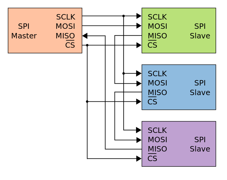
Figure 9-5. SPI configuration with three daisy-chained slaves

You will notice from pinout diagrams that some pins will be labelled with the names of SPI connections (SCLK, MOSI, MISO, etc.). Use these pins to attach SPI devices. Since there is an indeterminate number of CS connections, depending on how you are organising signalling, the CS pin should be selected and controlled by you. As with UART, each device is slightly different in terms of the steps to configure your SPI connections, although they are conceptually very similar. As before, you should consult the API documents for your device for the specific details. Nevertheless, the following REPL-based example for the PyBoard illustrates the essential steps you’ll need to take to make things work:

>>> from machine import SPI, Pin
>>> spi = SPI('X')
>>> cs = Pin('X1', Pin.OUT)
>>> cs.value(0)
>>> buffer = bytearray(5) 
>>> spi.write_readinto(b'hello', buffer)
>>> cs.value(1)

An spi object is instantiated with an indication of its position (there are two orientations for using SPI on the PyBoard: “X” and “Y”). The SPI class assumes the device will act as the master. A cs object is also instantiated from the Pin class to represent the chip select connection that is arbitrarily using the pin “X1” (see the PyBoard pinout to locate this pin). Note how it is set as an output. Pulling the cs object to low (0) indicates that any further interactions target the slave device connected to the chip select pin. A bytearray buffer is created for sending and receiving data. This must be the same size as the data to be sent. The message is sent and a response received into the buffer by calling the write_readinto method. Finally, the chip select connection is returned to high (1), indicating the end of the interaction.

In case you are wondering what bytes to send to SPI-connected peripherals in order to make them do something useful, or what their responses may mean, you should look at the manufacturer’s data sheet for the device. It’s important to note that, more often than not, the MicroPython community will have created a module that abstracts away the SPI communication for a particular device to allow you to concentrate on the “business logic” of your application rather than SPI-related implementation details. A good example is the lcd160cr module for the PyBoard that we used in an earlier chapter to drive the LCD colour display.

I²C

The inter-integrated circuit (I²C) protocol is the final hardware protocol you are likely to encounter with MicroPython.

Why another protocol? The answer can be found by looking at some of the drawbacks of UART or SPI.

With UART you are limited to a one-to-one connection and the overhead needed to mitigate problems with the asynchronous nature of the protocol. With SPI you require at least four connections (and potentially a lot more if you use several slave devices).

With I²C you only need two physical connections like UART, but those two wires could support many slave devices like SPI. Furthermore, I²C is capable of supporting a multiple master system whereby the master devices take it in turn to communicate with the slaves connected to the bus.

However, I²C isn’t capable of SPI’s speed of data transmission, so devices that need speedy data transfers will often use SPI rather than I²C. Both I²C and SPI are capable of much faster rates of data transfer than UART.

The two connections used by I²C are called SCL (for the clock signal) and SDA (for the data). The clock signal always comes from the current master. The connections for I²C are open drain, meaning they are pulled high by default, and devices change the signal by pulling low. This avoids the potential collision of a device driving the signal high while another is trying to pull it low (eliminating a situation where conflicting devices may cause damage to each other).

The protocol sent down the wire is more complicated than UART or SPI. Messages contain two parts: an address frame that indicates for whom the subsequent data is intended, and one or more data frames containing the actual data.

Communication is initiated by the master leaving the SCL connection high while pulling SDA low. This alerts the slave devices that a new message is about to be sent. The address frame is always the first thing sent in a new message and consists of a 7-bit address identifying the target slave, followed by a bit to indicate if the message is a read (1) or write (0). A ninth bit is used to allow the target slave to acknowledge receipt of the address frame. To do this, the target slave must pull the SDA line low before the ninth clock pulse. If this acknowledgment doesn’t happen, the exchange halts, and it’s up to the master to decide how to proceed.

Assuming a successful acknowledgment of the address frame, the subsequent data frames are synchronised by the master sending clock pulses via SCL, with the actual data transmitted via SDA by either the master or target slave (depending on if this is a read or write operation). The number of subsequent data frames is arbitrary in length and only stops when the master generates a stop condition: first SCL moves from low to high and remains high while SDA also moves from low to high.

While this may sound more complicated than SPI in terms of implementation details (it is), the end result is very easy to use from a programmatic point of view. Again, the caveats about different boards working slightly differently whilst being conceptually similar apply. Here is a REPL session as if using a PyBoard. The example assumes the connections as per the board’s pinout diagram for SCL and SDA connections:

>>> from machine import I2C
>>> i2c = I2C('X')
>>> i2c.scan()
[46]
>>> i2c.writeto(46, b'A')
1
>>> i2c.readfrom(46, 8)
b'x00Ax00Ax00Ax00A'
>>> i2c.writeto_mem(46, 0, b'A')
>>> i2c.readfrom_mem(46, 0, 2)
b'x00A'

In a fashion similar to the SPI example earlier, an i2c object is instantiated with an indication of the orientation. The I2C class assumes the device will act as a master. Since there could be several devices connected to the I²C bus, it’s possible to scan for their addresses (yielding a single device with the address 46). All subsequent communication uses this address to indicate the target device for instructions. The writeto and readfrom methods work as expected (sending a byte representation of “A” and receiving 8 bytes in return). The remaining two lines demonstrate how to write to and read from a particular memory address (indicated by 0) on a specific device (with the address 46).

As with SPI, you probably won’t need to directly use I²C since MicroPython will provide modules for specific devices that wrap all the implementation details. However, if you do need to drop to the I²C level, you should consult the data sheet from the manufacturer of the attached peripheral to discover what messages are used to interact with the device.

Miscellaneous GPIO Techniques and Protocols

The topics covered so far in this chapter give you a good foundation of knowledge about GPIO and should cover most of your GPIO-related interactions. However, sometimes you will encounter something a little more esoteric, so this final section will examine some of the darker corners to cover such cases.

Bit banging sounds like a nerdy version of whack-a-mole. It’s actually a lot more fun: it’s when you ignore hardware protocols and use software to control pins, timing, levels, and synchronisation in order to create a low-cost, highly bespoke solution to a peripheral-related problem. To say that it’s a “hack” is an understatement, but that’s what makes it such fun. So if you hear of someone mentioning bit banging, what they really mean is that they’re going “off piste” with code in terms of interactions with the hardware. Given the usually bespoke or experimental nature of a bit banging hack, the only common ground to describe here is that everything is controlled by the software, as needs apply, be that sampling, timing, controlling the signal, buffering, and so on. It’s the embedded version of poking with a stick to see what happens until you’ve figured it out. Why would you do such a thing? Sometimes it’s the simplest solution and reduces the overhead of complex code or allows you to abandon a large library (where you’re using only a small subset of its capabilities) in order to save precious space or resources.

Some peripherals don’t use UART, SPI, or I²C and have their own bespoke protocol. NeoPixels (also known as ws2812) and the digital humidity and temperature (DHT) line of sensors all use a 1-wire interface. These are just a couple of common examples you may run across and the actual implementation details are unimportant since MicroPython already has modules for both types of device. The point is that sometimes you may encounter a peripheral where none of the standard protocols apply and, if there’s no module already available, you may need to roll up your sleeves and get bit banging to make the thing blink or go bloop.

Perhaps the most enjoyable aspect of programming GPIO pins with MicroPython is that you’re close to the hardware. As Python programmers we’re used to working in relatively abstract computing environments where Python collaborates with the operating system to make things work. In contrast, as embedded developers, working in MicroPython retains the closeness to the hardware while giving us a high-level, expressive, and easy-to-use language that allows us to create working solutions in only a fraction of the time it would take in other, lower-level languages. The lack of abstractions and simplicity combined with the expressiveness of Python is a clue as to why MicroPython is such an exceptional teaching tool: you’re close enough to the hardware to be mucking about with how a computer actually works (rather than sitting on top of layers upon layers of abstractions), yet you have a powerful, flexible, and (most importantly) easy-to-learn programming language. That the skills learned with MicroPython are easily transferrable to “regular” Python is a testament to the continuity of experience that the Python ecosystem provides.