You learned Python in the preceding chapter. Now it is time to learn PySpark and utilize the power of a distributed system to solve problems related to big data. We generally distribute large amounts of data on a cluster and perform processing on that distributed data.
- This chapter covers the following recipes:
- Recipe 4-1. Create an RDD
- Recipe 4-2. Convert temperature data
- Recipe 4-3. Perform basic data manipulation
- Recipe 4-4. Run set operations
- Recipe 4-5. Calculate summary statistics
- Recipe 4-6. Start PySpark shell on Standalone cluster manager
- Recipe 4-7. Start PySpark shell on Mesos
- Recipe 4-8. Start PySpark shell on YARN
Learning about the architecture of Spark will be very helpful to your understanding of the various components of Spark. Before delving into the recipes let’s explore this topic.
Figure 4-1 describes the Spark architecture.
Figure 4-1.
Spark architecture
The main components of the Spark architecture are the driver and executors. For each PySpark application, there will be one driver program and one or more executors running on the cluster slave machine. You might be wondering, what is an application in the context of PySpark? An application is a whole bunch of code used to solve a problem.
The
driver
is the process that coordinates with many executors running on various slave machines. Spark follows a master/slave architecture. The SparkContext object is created by the driver. SparkContext is the main entry point to a PySpark application. You will learn more about SparkContext in upcoming chapters. In this chapter, we will run our PySpark commands in the PySpark shell. After starting the shell, we will find that the SparkContext object is automatically created. We will encounter the SparkContext object in the PySpark shell as the variable sc. The shell itself is working as our driver. The driver breaks our application into small tasks; a task is the smallest unit of your application. Tasks are run on different executors in parallel. The driver is also responsible for scheduling tasks to different executors.
Executors
are slave processes. An executor runs tasks. It also has the capability to cache data in memory by using the BlockManager process. Each executor runs in its own Java Virtual Machine (JVM).
The cluster manager manages cluster resources. The driver talks to the cluster manager to negotiate resources. The cluster manager also schedules tasks on behalf of the driver on various slave executor processes. PySpark is dispatched with Standalone Cluster Manager. PySpark can also be configured on YARN and Apache Mesos. In our recipes, you are going to see how to configure PySpark on Standalone Cluster Manager and Apache Mesos. On a single machine, PySpark can be started in local mode too.
The main celebrated component of PySpark is the resilient distributed dataset (RDD). The RDD is a data abstraction over the distributed collection. Python collections such as lists, tuples, and sets can be distributed very easily. An RDD is recomputed on node failures. Only part of the data is calculated or recalculated, as required. An RDD is created using various functions defined in the
SparkContext
class. One important method for creating an RDD is parallelize(), which you will encounter again and again in this chapter. Figure 4-2 illustrates the creation of an RDD.
Figure 4-2.
Creating an RDD
Let’s say that we have a Python collection with the elements Data1, Data2, Data3, Data4, Data5, Data6, and Data7. This collection is distributed over the cluster to create an RDD. For simplicity, we can assume that two executors are running. Our collection is divided into two parts. The first executor gets the first part of the collection, which has the elements Data1, Data2, Data3, and Data4. The second part of the collection is sent to the second executor. So, the second executor has the data elements Data5, Data6, and Data7.
We can perform two types of operations on the RDD: transformation and action
. Transformation on an RDD returns another RDD. We know that RDDs are immutable; therefore, changing the RDD is impossible. Hence transformations always return another RDD. Transformations are lazy, whereas actions are eagerly evaluated. I say that the transformation is lazy because whenever a transformation is applied to an RDD, that operation is not applied to the data at the same time. Instead, PySpark notes the operation request, but all the transformations are applied when the first action is called.
Figure 4-3 illustrates a transformation
operation. The transformation on RDD1 creates RDD2. RDD1 has two partitions. The first partition of RDD1 has four data elements: Data1, Data2, Data3, and Data4. The second data partition of RDD1 has three elements: Data5, Data6, and Data7. After transformation on RDD1, RDD2 is created. RDD2 has six elements. So it is clear that the daughter RDD might have a different number of data elements than the father RDD. RDD2 also has two partitions. The first partition of RDD2 has three data points: Data8, Data9, and Data10. The second partition of RDD2 also has three elements: Data11, Data12, and Data13. Don’t get confused about the daughter RDD having a different number of partitions than the father RDD. 
Figure 4-3.
RDD transformations
Figure 4-4 illustrates an action performed on an RDD. In this example, we are applying the summation action. Summed data is returned to the driver. In other cases, the result of an action can be saved to a file or to another destination.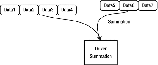
Figure 4-4.
RDD action
You might be wondering, if Spark has been written in Scala, then how is Python contacting with Scala? You might guess that a Python wrapper of PySpark has been written using Jython, and that this Jython code is compiled to Java bytecode and run on the JVM. This guess isn’t correct.
A running Python program can access Java objects in a JVM by using Py4J. A running Java program can also access Python objects by using Py4J. A gateway between Python and Java enables Python to use Java objects.
Driver programs use Py4J to communicate between Python and the Java SparkContext object. PySpark uses Py4J, so that PySpark Python code can
On remote cluster machines, the PythonRDD object creates Python subprocesses and communicates with them using pipes. The PythonRDD object runs in JVM and communicates with Python processes by using pipes.
Note
You can learn more about Py4J at the following locations:
Recipe 4-1. Create an RDD
Problem
You want to create an RDD.
Solution
As we know, an RDD is a distributed collection. You have a list with the following data:
pythonList = [2.3,3.4,4.3,2.4,2.3,4.0]
You want to do the following operations:
- Create an RDD of the list
- Get the first element
- Get the first two elements
- Get the number of partitions in the RDD
In PySpark, an RDD can be created in many ways. One way to create an RDD out of a given collection is to use the
parallelize()
function. The SparkContext object is used to call the parallelize() function. You’ll read more about SparkContext in an upcoming chapter.
In the case of big data, even tabular data, a table might have more than 1,000 columns. Sometimes analysts want to see what those columns of data look like. The first() function is defined on an RDD and will return the first element of the RDD.
To get more than one element from a list, we can use the take() function. The number of partitions of a collection can be fetched by using getNumPartitions().
How It Works
Let’s follow the steps in this section to solve the problem.
Step 4-1-1. Creating an RDD of the List
Let’s first create a Python list by using the following:
>>> pythonList = [2.3,3.4,4.3,2.4,2.3,4.0]
>>> pythonList
Here is the output:
[2.3, 3.4, 4.3, 2.4, 2.3, 4.0]
Parallelization or distribution of data is done using the parallelize() function. This function takes two arguments. The first argument is the collection to be parallelized, and the second argument indicates the number of distributed chunks of data you want:
>>> parPythonData = sc.parallelize(pythonList,2)
Using the parallelize() function, we have distributed our data in two partitions. In order to get all the data on the driver, we can use the collect() function, as shown in the following code line. Using the collect() function is not recommended in production; rather, it should be used only in code debugging.
>>> parPythonData.collect()
Here is the output:
[2.3, 3.4, 4.3, 2.4, 2.3, 4.0]
Step 4-1-2. Getting the First Element
The
first()
function can be used to get the first data out of an RDD. You might have figured out that the collect() and first() functions perform actions:
>>> parPythonData.first()
Here is the output:
2.3
Step 4-1-3. Getting the First Two Elements
Sometimes data analysts want to see more than one row of data. The
take()
function can be used to fetch more than one row from an RDD. The number of rows you want is given as an argument to the take() function:
>>> parPythonData.take(2)
Here is the output:
[2.3, 3.4]
Step 4-1-4. Getting the Number of Partitions in the RDD
In order to optimize PySpark code, a proper distribution of data is required. The number of partitions of an RDD can be found using the
getNumPartitions()
function:
>>> parPythonData.getNumPartitions()
Here is the output:
2
Recall that we were partitioning our data into two partitions while using the parallelize() function.
Recipe 4-2. Convert Temperature Data
Problem
You want to convert temperature data by writing a temperature unit conversion program on an RDD.
Solution
You are given daily temperatures in Fahrenheit. You want to perform some analysis on that data. But your new software takes input in Celsius. Therefore, you want to convert your temperature data
from Fahrenheit to Celsius. Table 4-1 shows the data you have.
Table 4-1.
Daily Temperature in Fahrenheit
You want to do the following:
- Convert temperature from Fahrenheit to Celsius
- Get all the temperature data points greater than 13o C
We can convert temperature from Fahrenheit to Celsius by using the following mathematical formula:
oC = (oF – 32) × 5/9
We can see that in PySpark, this is a transformation problem. We can achieve this task by using the map() function on the RDD.
Getting all the temperatures greater than 13o C is a filtering problem. Filtering of data can be done by using the filter() function on the RDD.
How It Works
We’ll follow the steps in this section to complete the conversion and filtering exercises.
Step 4-2-1. Parallelizing the Data
We are going to parallelize data by using our parallelize() function. We are going to distribute our data in two partitions, as follows:
>>> tempData = [59,57.2,53.6,55.4,51.8,53.6,55.4]
>>> parTempData = sc.parallelize(tempData,2)
>>> parTempData.collect()
Here is the output:
[59, 57.2, 53.6, 55.4, 51.8, 53.6, 55.4]
The collection of data has returned our parallelized data.
Step 4-2-2. Converting Temperature from Fahrenheit to Celsius
Now we are going to convert our temperature in Fahrenheit to Celsius. We’ll write a fahrenheitToCentigrade function, which will take the temperature in Fahrenheit and return a temperature in Celsius for a given input:
>>> def fahrenheitToCentigrade(temperature) :
... centigrade = (temperature-32)*5/9
... return centigrade
Let’s test our fahrenheitToCentigrade function:
>>> fahrenheitToCentigrade(59)
Here is the output:
15
We are providing 59 as the input in Fahrenheit. Our function returns a Celsius value of our Fahrenheit input; 59o F is equal to 15o C.
>>> parCentigradeData = parTempData.map(fahrenheitToCentigrade)
>>> parCentigradeData.collect()
Here is the output:
[15, 14.000000000000002, 12.0, 13.0, 10.999999999999998, 12.0, 13.0]
We have converted the given temperature to Celsius. Now let’s filter out all the temperatures greater than or equal to 13o C.
Step 4-2-3. Filtering Temperatures Greater than 13o C
To filter data, we can use the filter() function on the RDD. We have to provide a predicate as input to the filter() function. A predicate is a function that tests a condition and returns True or False.
Let’s define the predicate tempMoreThanThirteen, which will take a temperature value and return True if input is greater than or equal to 13:
>>> def tempMoreThanThirteen(temperature):
... return temperature >=13
We are going to send our tempMoreThanThirteen function as input to the filter() function. The filter() function will iterate over each value in the parCentigradeData RDD. For each value, the tempMoreThanThirteen function will be applied. If the value is greater than or equal to 13, True will be returned. The value for which tempMoreThanThirteen returns True will come to filteredTemprature:
>>> filteredTemprature = parCentigradeData.filter(tempMoreThanThirteen)
>>> filteredTemprature.collect()
Here is the output:
[15, 14.000000000000002, 13.0, 13.0]
We can replace our predicates by using the lambda function. (We discussed lambda functions in Chapter 3.) Using a lambda function makes the code more readable. The following code line clearly depicts that the filter() function takes a predicate as input and returns True for all the values greater than or equal to 13:
>>> filteredTemprature = parCentigradeData.filter(lambda x : x>=13)
>>> filteredTemprature.collect()
Here is the output:
[15, 14.000000000000002, 13.0, 13.0]
We finally have four elements indicating a temperature that is either greater than or equal to 13. So now you understand the way to do basic analysis on data with PySpark
.
Recipe 4-3. Perform Basic Data Manipulation
Problem
You want to do data manipulation and run aggregation operations.
Solution
In this recipe, you are given data indicating student grades for a two-year (four-semester) course. Seven students are enrolled in this course. Table 4-2 depicts two years of grade data, divided into semesters, for seven enrolled students.
Table 4-2.
Student Grades
You want to calculate the following:
- Average grades per semester, each year, for each student
- Top three students who have the highest average grades in the second year
- Bottom three students who have the lowest average grades in the second year
- All students who have earned more than an 80% average in the second semester of the second year
Using the
map()
function is often helpful. In this example, the average grades per semester, for each year, can be calculated using map().
It is a general data science problem to get the top k elements, such as the top k highly performing bonds. The PySpark takeOrdered() function is going to take the top k or top bottom elements from our RDD.
Students who have earned more than 80% averages in the second year can be filtered using the filter() function.
How It Works
Let’s solve our problem in steps. We will start with creating an RDD of our data.
Step 4-3-1. Making a List from a Given Table
In this step, we’ll create a nested list
. This means that each element of the list is a record, and each record is a list in itself:
>>> studentMarksData = [["si1","year1",62.08,62.4],
... ["si1","year2",75.94,76.75],
... ["si2","year1",68.26,72.95],
... ["si2","year2",85.49,75.8],
... ["si3","year1",75.08,79.84],
... ["si3","year2",54.98,87.72],
... ["si4","year1",50.03,66.85],
... ["si4","year2",71.26,69.77],
... ["si5","year1",52.74,76.27],
... ["si5","year2",50.39,68.58],
... ["si6","year1",74.86,60.8],
... ["si6","year2",58.29,62.38],
... ["si7","year1",63.95,74.51],
... ["si7","year2",66.69,56.92]]
Step 4-3-2. Parallelizing the Data
After parallelizing the data by using the parallelize() function, we will find that we have an RDD in which each element is a list itself:
>>> studentMarksDataRDD = sc.parallelize(studentMarksData,4)
As we know, the collect() function takes the whole RDD to the driver. If the RDD size is very large, the driver may face a memory issue. In order to fetch k first elements of an RDD, we can use the
take()
function with n as input to take(). As an example, in the following line of code, we are fetching two elements of our RDD. Remember here that take() is an action:
>>> studentMarksDataRDD.take(2)
Here is the output:
[['si1', 'year1', 62.08, 62.4],
['si1', 'year2', 75.94, 76.75]]
Step 4-3-3. Calculating Average Semester Grades
Now let me explain what I want to do in the following code. Just consider the first element of the RDD. Our first element of the RDD is ['si1', 'year1', 62.08, 62.4], which is a list of four elements. Our work is to calculate the mean of grades from two semesters. In the first element, the mean is 0.5(62.08 + 62.4). We are going to use the
map()
function to get our solution.
>>> studentMarksMean = studentMarksDataRDD.map(lambda x : [x[0],x[1],(x[2]+x[3])/2])
Again, we use the take() function to visualize the map() function output:
>>> studentMarksMean.take(2)
Here is the output:
[['si1', 'year1', 62.239999999999995],
['si1', 'year2', 76.345]]
Step 4-3-4. Filtering Student Average Grades in the Second Year
The following line of code is going to filter out all the data of the second year. We have implemented our predicate by using a lambda function. Our predicate function checks whether year2 is in the list. If the predicate returns True, the list includes second-year grades.
>>> secondYearMarks = studentMarksMean.filter(lambda x : "year2" in x)
>>> secondYearMarks.take(2)
Here is the output:
[['si1', 'year2', 76.345],
['si2', 'year2', 80.645]]
We can clearly see that the RDD output of secondYearMarks has only second-year grades.
Step 4-3-5. Finding the Top Three Students
We can get the top three students in two ways. The first method is to sort the full data according to grades. Obviously, we are going to sort the data in decreasing order. Sorting is done by the sortBy() function. Let’s see the implementation:
>>> sortedMarksData = secondYearMarks.sortBy(keyfunc = lambda x : -x[2])
In our
sortBy()
function, we provide the keyfunc parameter. This parameter indicates to sort the grades data in decreasing order. Now collect the output and see the result:
>>> sortedMarksData.collect()
Here is the output:
[['si2', 'year2', 80.645],
['si1', 'year2', 76.345],
['si3', 'year2', 71.35],
['si4', 'year2', 70.515],
['si7', 'year2', 61.805],
['si6', 'year2', 60.335],
['si5', 'year2', 59.485]]
After sorting data, we can take the first three elements by using our take() function:
>>> sortedMarksData.take(3)
Here is the output:
[['si2', 'year2', 80.645],
['si1', 'year2', 76.345],
['si3', 'year2', 71.35]]
We have our answer. But can we optimize it further? In order to get top-three data, we are sorting the whole list. We can optimize this by using the takeOrdered() function. This function takes two arguments: the number of elements we require, and key, which uses a lambda function to determine how to take the data out.
>>> topThreeStudents = secondYearMarks.takeOrdered(num=3, key = lambda x :-x[2])
In the preceding code, we set num to 3 for the three top elements, and lambda in key so that it can provide three top in decreasing order.
>>> topThreeStudents
Here is the output:
[['si2', 'year2', 80.645],
['si1', 'year2', 76.345],
['si3', 'year2', 71.35]]
In order to print the result, we are not using the
collect()
function to get the data. Remember that transformation creates another RDD, so we require the collect() function to collect data. But an action will directly fetch the data to the driver, and collect() is not required. So you can conclude that the takeOrdered() function is an action.
Step 4-3-6. Finding the Bottom Three Students
We have to find the bottom three students in terms of their average grades. One way is to sort the data in increasing order and take the three on top. But that is not an efficient way, so we will use the takeOrdered() function again, but with a different key parameter:
>>> bottomThreeStudents = secondYearMarks.takeOrdered(num=3, key = lambda x :x[2]])
>>> bottomThreeStudents
Here is the output:
[['si5', 'year2', 59.485],
['si6', 'year2', 60.335],
['si7', 'year2', 61.805]]
Step 4-3-7. Getting All Students with 80% Averages
Now that you understand the
filter()
function, it is easy to guess that we can solve this problem by using filter(). We will have to provide a predicate, which will return True if grades are greater than 80; otherwise, it returns False.
>>> moreThan80Marks = secondYearMarks.filter(lambda x : x[2] > 80)
>>> moreThan80Marks.collect()
Here is the output:
[['si2', 'year2', 80.645]]
It can be observed that only one student (with the student ID si2) has secured more than an 80% average in the second year.
Recipe 4-4. Run Set Operations
Problem
You want to run set operations
on a research company’s data.
Solution
XYZ Research is a company that performs research on many diversified topics. Each research project comes with a research ID. Research may come to a conclusion in one year or may take more than one year. The following data is provided, indicating the number of research projects being conducted in three years:
2001: RIN1, RIN2, RIN3, RIN4, RIN5, RIN6, RIN7
2002: RIN3, RIN4, RIN7, RIN8, RIN9
2003: RIN4, RIN8, RIN10, RIN11, RIN12
Now we have to answer the following questions:
- How many research projects were initiated in the three years?
- How many projects were completed in the first year?
- How many projects were completed in the first two years?
A set is collection of distinct elements. PySpark performs pseudo set operations. They are called pseudo set operations because some functions do not remove duplicate elements.
Remember, the first question is not asking about completed projects. The total number of research projects initiated in three years is just the union of all three years of data. You can perform a union on two RDDs by using the union() function.
The projects that have been started in the first year and not in the second year are the projects that have been completed in the first year. Every project that is started is completed. We can use the subtract() function to find all the projects that were completed in the first year.
If we make a union of first-year and second-year projects and subtract third-year projects, we are going to get all the projects that have been completed in the first two years.
How It Works
Let’s solve this problem step-by-step
.
Step 4-4-1. Creating a List of Research Data by Year
Let’s start with creating a list of all the projects that the company worked on each year:
>>> data2001 = ['RIN1', 'RIN2', 'RIN3', 'RIN4', 'RIN5', 'RIN6', 'RIN7']
>>> data2002 = ['RIN3', 'RIN4', 'RIN7', 'RIN8', 'RIN9']
>>> data2003 = ['RIN4', 'RIN8', 'RIN10', 'RIN11', 'RIN12']
data2001 is list of all the projects started in 2001. Similarly, data2002 contains all the research projects that either are continuing from 2001 or started in 2002. The data2003data list contains all the projects that the company worked on in 2003.
Step 4-4-2. Parallelizing the Data (Creating the RDD)
After creating lists, we have to parallelize our data:
>>> parData2001 = sc.parallelize(data2001,2)
>>> parData2002 = sc.parallelize(data2002,2)
>>> parData2003 = sc.parallelize(data2003,2)
After parallelizing, we get three RDDs. The first RDD is parData2001, the second RDD is parData2002, and the last one is parData2003.
Step 4-4-3. Finding Projects Initiated in Three Years
The total number of projects initiated in three years is determined just by getting the union of all the data for the given three years. RDD union() takes another RDD as input and returns, merging these two RDDs. Let’s see how it works:
>>> unionOf20012002 = parData2001.union(parData2002)
>>> unionOf20012002.collect()
Here is the output:
['RIN1', 'RIN2', 'RIN3', 'RIN4',
'RIN5', 'RIN6', 'RIN7', 'RIN3',
'RIN4', 'RIN7', 'RIN8', 'RIN9']
We have calculated the union of different research projects initiated in either the first year or the second year. We can observe that the unionized data, unionOf20012002, has duplicate values. Having duplicates values in sets is not allowed. Therefore, a set operation on an RDD is also known as a pseudo set operation. Don’t worry; we will remove these duplicates.
In order to get all the research projects that have been initiated in three years, we have to get the union of parData2003 and unionOf20012002:
>>> allResearchs = unionOf20012002.union(parData2003)
>>> allResearchs.collect()
Here is the output:
['RIN1', 'RIN2', 'RIN3', 'RIN4',
'RIN5', 'RIN6', 'RIN7', 'RIN3',
'RIN4', 'RIN7', 'RIN8', 'RIN9',
'RIN4', 'RIN8', 'RIN10', 'RIN11', 'RIN12']
We have the union of all three years of data
. Now we have to get rid of duplicates.
Step 4-4-4. Making Sets of Distinct Data
We are going to apply the distinct() function to our RDD allResearchs:
>>> allUniqueResearchs = allResearchs.distinct()
>>> allUniqueResearchs.collect()
Here is the output:
['RIN1', 'RIN12', 'RIN5', 'RIN3',
'RIN4', 'RIN2', 'RIN11', 'RIN7',
'RIN9', 'RIN6', 'RIN8', 'RIN10']
We can see that we have all the research projects that were initiated in the first three years.
Step 4-4-5. Counting Distinct Elements
Now count all the distinct research projects by using the count() function on the RDD:
>>> allResearchs.distinct().count()
Here is the output:
12
Note
We can run telescopic commands in PySpark too.
The following command is run in telescopic fashion:
>>> parData2001.union(parData2002).union(parData2003).distinct().count()
Here is the output:
12
Step 4-4-6. Finding Projects Completed the First Year
Let’s say we have two sets, A and B. Subtracting set B from set A will give us all the elements that are members of set A but not set B. So now it is clear that, in order to know all the projects that have been completed in the first year (2001), we have to subtract the projects in year 2002 from all the projects in year 2001.
Subtraction on a set can be done with the subtract() function:
>>> firstYearCompletion = parData2001.subtract(parData2002)
>>> firstYearCompletion.collect()
Here is the output:
['RIN5', 'RIN1', 'RIN6', 'RIN2']
We have all the projects that were completed in 2001. Four projects were completed in 2001.
Step 4-4-7. Finding Projects Completed in the First Two Years
A union of RDDs gives us all the projects started in the first two years. After getting all the projects started in the first two years, if we then subtract projects running and started in the third year, we will return all the projects completed in the first two years. The following is the implementation:
>>> unionTwoYears = parData2001.union(parData2002)
>>> unionTwoYears.subtract(parData2003).collect()
Here is the output:
['RIN1', 'RIN5', 'RIN3', 'RIN3',
'RIN2', 'RIN7', 'RIN7', 'RIN9', 'RIN6']
Now subtract:
>>> unionTwoYears.subtract(parData2003).distinct().collect()
Here is the output:
['RIN1', 'RIN5', 'RIN3',
'RIN2', 'RIN7', 'RIN9', 'RIN6']
Step 4-4-8. Finding Projects Started in 2001 and Continued Through 2003.
This step requires using the intersection() method defined in PySpark on the RDD:
>>> projectsInTwoYear = parData2001.intersection(parData2002)
>>> projectsInTwoYear.collect()
Here is the output:
['RIN4', 'RIN7', 'RIN3']
>>> projectsInTwoYear.subtract(parData2003).distinct().collect()
Here is the output
:
['RIN3', 'RIN7']
Recipe 4-5. Calculate Summary Statistics
Problem
You want to calculate summary statistic
s on given data.
Solution
Renewable energy sources are gaining in popularity all over the world. The company FindEnergy wants to install windmills at a given location. For efficient operation of windmills, the air requires certain characteristics.
Data is collected as shown in Table 4-3.
Table 4-3.
Air Velocity Data
You, as a data scientist, want to calculate the following quantities:
- Number of data points
- Summation of air velocities over a day
- Mean air velocity in a day
- Variance of air data
- Sample variance of air data
- Standard deviation of air data
- Sample standard deviation of air data
PySpark provides many functions to summarize data on the RDD. The number of elements in an RDD can be found by using the count() function on the RDD. There are two ways to sum all the data in a given RDD. The first is to apply the sum() method to the RDD. The second is to apply the reduce() function to the RDD.
The mean represents the center point of the given data, and it can be calculated in two ways too. We are going to use the mean() method and the fold() method to calculate the mean.
The variance, which indicates the spread of data around the mean, can be calculated using the variance() function. Similarly, the sample variance can be calculated by using the sampleVariance() method on the RDD.
Standard deviation and sample standard deviation will be calculated using the stdev() and sampleStdev() methods, respectively.
PySpark provides the stats() method, which can calculate all the previously mentioned quantities in one go.
How It Works
We’ll follow the steps in this section to reach a solution.
Step 4-5-1. Parallelizing the Data
Let’s parallelize the air velocity data from a list:
>>> airVelocityKMPH = [12,13,15,12,11,12,11]
>>> parVelocityKMPH = sc.parallelize(airVelocityKMPH,2)
The parVelocityKMPH variable is an RDD.
Step 4-5-2. Getting the Number of Data Points
The number of data points gives us an idea of the data size. We apply the count() function to get the number of elements in the RDD:
>>>countValue = parVelocityKMPH.count()
Here is the output:
7
The total number of data points is seven.
Step 4-5-3. Summing Air Velocities in a Day
Let’s get the summation by using the sum() method:
>>>sumValue = parVelocityKMPH.sum()
Here is the output:
86
Step 4-5-4. Finding the Mean Air Velocity
Figure 4-5 shows the mathematical formula for finding a mean, where x1, x2, . . . xn are n data points.
Figure 4-5.
Calculating the mean
We calculate the mean by using the mean() function defined on the RDD:
>>>meanValue = parVelocityKMPH.mean()
Here is the output:
12.285714285714286
Step 4-5-5. Finding the Variance of Air Data
If we have the data points x1, x2, . . . xn, then Figure 4-6 shows the mathematical formula for calculating variance. We are going to calculate the variance of the given air data by using the variance() function defined on the RDD.
Figure 4-6.
Calculating the variance
>>> varianceValue = parVelocityKMPH.variance()
Here is the output:
1.63265306122449
Step 4-5-6. Calculating Sample Variance
The variance function calculates the population variance. In order to calculate the sample variance, we have to use sampleVariance() defined on the RDD.
For data points x1, x2, . . . xn, the sample standard variance is defined in Figure 4-7.
Figure 4-7.
Calculating the sample variance
The following line of code calculates the sample standard deviation:
>>> sampleVarianceValue = parVelocityKMPH.sampleVariance()
Here is the output:
1.904761904761905
Step 4-5-7. Calculating Standard Deviation
The standard deviation is the square root of the variance value. Let’s calculate the standard deviation by using the stdev() function:
>>> stdevValue = parVelocityKMPH.stdev()
Here is the output:
1.2777531299998799
The standard deviation of the given air velocity data is 1.2777531299998799.
Step 4-5-8. Calculating Sample Standard Deviation
>>> sampleStdevValue = parVelocityKMPH.sampleStdev()
Here is the output:
1.3801311186847085
Step 4-5-9. Calculating All Values in One Step
We can calculate all the values of the summary statistics in one go by using the stats() function. The StatCounter object is returned from the stats() function. Let’s use the stats() function to calculate the summary statistics of the air velocity data:
>>> type(parVelocityKMPH.stats())
Here is the output:
<class 'pyspark.statcounter.StatCounter'>
>>> parVelocityKMPH.stats()
Here is the output:
(count: 7, mean: 12.2857142857, stdev: 1.27775313, max: 15.0, min: 11.0)
We can see that the stats() function is an action. It calculates the count, mean, standard deviation, maximum, and minimum of an RDD in one go. It returns the result as a tuple with elements that are key/value pairs. The result of the stats() function can be transformed into a dictionary by using the asDict() function:
>>> parVelocityKMPH.stats().asDict()
Here is the output:
{'count': 7, 'min': 11.0, 'max': 15.0, 'sum': 86.0, 'stdev': 1.3801311186847085, 'variance': 1.904761904761905, 'mean': 12.285714285714286}
We also can get individual elements by using different functions defined on StatCounter. Let’s start with fetching the mean. The mean value can be found by using the mean() function defined on the StatCounter object:
>>> parVelocityKMPH.stats().mean()
Here is the output:
12.285714285714286
Similarly, we can get the number of elements in the RDD, the minimum value, the maximum value, and the standard deviation by using the functions count(), min(), max(), and stdev() functions, respectively. Let’s start with the standard deviation:
>>> parVelocityKMPH.stats().stdev()
Here is the output:
1.2777531299998799
This command provides the number of elements:
>>> parVelocityKMPH.stats().count()
Here is the output
:
7
Next, we find the minimum value:
>>> parVelocityKMPH.stats().min()
Here is the output:
11.0
Then we find the maximum value:
>>> parVelocityKMPH.stats().max()
Here is the output:
15.0
Recipe 4-6. Start PySpark Shell on Standalone Cluster Manager
Problem
You want to start PySpark shell using Standalone Cluster Manager
.
Solution
Standalone Cluster Manager provides a master/slave structure. In order to start Standalone Cluster Manager on a single machine, we can use the start-all.sh script. We can find this script inside $SPARK_HOME/sbin. In our case, $SPARK_HOME is /allPySpark/spark. In a cluster environment, we can run a master script to run the master on one machine, and a slave script on a different slave machine to start the slave.
We can start the PySpark shell by using the master URL of the Standalone master. The Standalone master URL looks like spark://<masterHostname>:<masterPort>. It can be easily found in the log file of the master
.
How It Works
We have to start the Standalone master and slave processes. There are two ways to do this. In the spark/sbin directory, we will find the start-all.sh script. It will start the master and slave together on the same machine.
Another way to start the processes is as follows: on the master machine, start the master by using the start-master.sh script; and start the slave on a different machine by using start-slave.sh.
Step 4-6-1. Starting Standalone Cluster Manager Using the start-all.sh Script
In this step, we are going to run the start-all.sh script:
[pysparkbook@localhost ∼]$ /allPySpark/spark/sbin/start-all.sh
Here is the output:
starting org.apache.spark.deploy.master.Master, logging to /allPySpark/logSpark//spark-pysparkbook-org.apache.spark.deploy.master.Master-1-localhost.localdomain.out
localhost: starting org.apache.spark.deploy.worker.Worker, logging to /allPySpark/logSpark//spark-pysparkbook-org.apache.spark.deploy.worker.Worker-1-localhost.localdomain.out
The logs of starting the Standalone cluster by using the start-all.sh script are written to two files. The file spark-pysparkbook-org.apache.spark.deploy.master.Master-1-localhost.localdomain.out is the log of starting the master process. In order to connect to the master, we need the master URL. We can find this URL in the log file.
Let’s open the master log file:
[pysparkbook@localhost ∼]$ vim /allPySpark/logSpark//spark-pysparkbook-org.apache.spark.deploy.master.Master-1-localhost.localdomain.out
Here is the output:
17/03/02 03:33:59 INFO util.Utils: Successfully started service 'sparkMaster' on port 7077.
17/03/02 03:33:59 INFO master.Master: Starting Spark master at spark://localhost.localdomain:7077
17/03/02 03:33:59 INFO master.Master: Running Spark version 1.6.2
17/03/02 03:34:10 INFO server.Server: jetty-8.y.z-SNAPSHOT
17/03/02 03:34:10 INFO server.AbstractConnector: Started [email protected]:8080
17/03/02 03:34:10 INFO util.Utils: Successfully started service 'MasterUI' on port 8080.
17/03/02 03:34:10 INFO ui.MasterWebUI: Started MasterWebUI at http://10.0.2.15:8080
The logs in the master log file indicate that the master has been started on spark://localhost.localdomain:7077 and that the master web UI is at http://10.0.2.15:8080.
Let’s open the master web UI, shown in Figure 4-8. In this UI, we can see the URL of the Standalone master
.
Figure 4-8.
Spark master
The following command will start the PySpark shell on the Standalone cluster:
[pysparkbook@localhost ∼]$/allPySpark/spark/bin/pyspark --master spark://localhost.localdomain:7077
After running jps, we can see the master and worker processes:
[pysparkbook@localhost ∼]$ jps
Here is the output
:
4246 Worker
3977 Master
4285 Jps
We can stop Standalone Cluster Manager by using the stop-all.sh script:
[pysparkbook@localhost ∼]$ /allPySpark/spark/sbin/stop-all.sh
Here is the output:
localhost: stopping org.apache.spark.deploy.worker.Worker
stopping org.apache.spark.deploy.master.Master
We can see that the stop-all.sh script first stops the worker (slave) and then stops the master.
Step 4-6-2. Starting Standalone Cluster Manager with an Individual Script
The PySpark framework provides an individual script for starting the master and workers on different machines. Let’s first start the master by using the start-master.sh script:
[pysparkbook@localhost ∼]$ /allPySpark/spark/sbin/start-master.sh
Here is the output:
starting org.apache.spark.deploy.master.Master, logging to /allPySpark/logSpark//spark-pysparkbook-org.apache.spark.deploy.master.Master-1-localhost.localdomain.out
Again, as done previously, we have to get the master URL from the log file. Using that master URL, we can start slaves on different machines by using the start-slave.sh script:
[pysparkbook@localhost ∼]$ /allPySpark/spark/sbin/start-slave.sh spark://localhost.localdomain:7077
Here is the output:
starting org.apache.spark.deploy.worker.Worker, logging to /allPySpark/logSpark//spark-pysparkbook-org.apache.spark.deploy.worker.Worker-1-localhost.localdomain.out
Using the jps command, we can see the worker and master processes running on our machine:
[pysparkbook@localhost ∼]$ jps
Here is the output:
4246 Worker
3977 Master
4285 Jps
You might remember that when we use stop-all.sh, the script first stops the worker process and then the master process. We have to follow this order. We stop the worker process first, followed by the master process.
To stop the worker process, use the stop-slave.sh script:
[pysparkbook@localhost ∼]$ /allPySpark/spark/sbin/stop-slave.sh
Here is the output:
stopping org.apache.spark.deploy.worker.Worker
Running the jps command will show only the master process now:
[pysparkbook@localhost ∼]$ jps
Here is the output:
4341 Jps
3977 Master
Similarly, we can stop the master process by using the stop-master.sh script:
[pysparkbook@localhost ∼]$ /allPySpark/spark/sbin/stop-master.sh
Here is the output:
stopping org.apache.spark.deploy.master.Master
Recipe 4-7. Start PySpark Shell on Mesos
Problem
You want to start PySpark shell on a Mesos cluster manager
.
Solution
Mesos is another cluster manager. Mesos also follows a master/slave architecture, similar to Standalone Cluster Manager. In order to start Mesos, we have to first start the Mesos master and then the Mesos slave. Then the PySpark shell can be started by using the master URL on Mesos.
How It Works
We installed Mesos in Chapter 3. Now we have to start the master and slave processes one by one. After starting the master and slaves, we have to start the PySpark shell. The following command starts the Mesos master process:
[pysparkbook@localhost ∼]$ mesos-master –work_dir=/allPySpark/mesos/workdir
Here is the output:
I0224 09:50:57.575908 9839 main.cpp:263] Build: 2016-12-29 00:42:08 by pysparkbook
I0224 09:50:57.576501 9839 main.cpp:264] Version: 1.1.0
I0224 09:50:57.582787 9839 main.cpp:370] Using 'HierarchicalDRF' allocator
The slave process will start subsequent to the start of the master process:
[root@localhost binaries]#mesos-slave --master=127.0.0.1:5050 --work_dir=/allPySpark/mesos/workdir1 --systemd_runtime_directory=/allPySpark/mesos/systemd
Here is the output:
I0224 18:22:25.002970 3797 gc.cpp:55] Scheduling '/allPySpark/mesos/workdirSlave/slaves/dd2c5f22-57f9-416e-a71a-0cc83de8558d-S1/frameworks/dd2c5f22-57f9-416e-a71a-0cc83de8558d-0000/executors/1/runs/a7c3d613-9696-4d42-afe2-a27c5c825e72' for gc 6.99998839417778days in the future
I0224 18:22:25.003083 3797 gc.cpp:55] Scheduling
I0224 18:22:25.003123 3797 gc.cpp:55] Scheduling '/allPySpark/mesos/workdirSlave/slaves/dd2c5f22-57f9-416e-a71a-0cc83de8558d-S1/frameworks/dd2c5f22-57f9-416e-a71a-0cc83de8558d-0000' for gc 6.99998839205926days in the future
We have our master and slave processes started. Now we can start the PySpark shell by using the following command. We provide the master URL and one parameter, spark.executor.uri. The spark.executor.uri parameter tells Mesos the location to get the PySpark assembly.
[pysparkbook@localhost binaries]$ /allPySpark/spark/bin/pyspark --master mesos://127.0.0.1:5050 --conf spark.executor.uri=/home/pysparkbook/binaries/spark-2.0.0-bin-hadoop2.6.tgz
We can run the jps command to see the Java process
after running PySpark on Mesos:
[pysparkbook@localhost binaries]$jps
Here is the output:
4174 SparkSubmit
4287 CoarseGrainedExecutorBackend