This chapter gives some examples of flow control as well as ways to do the examples using indexing. The first example uses nested for loops and if/else statements. The second example uses the while statement. The third example is of nested for loops. The fourth example uses a for loop, an if statement, and a next statement. The fifth example is of a for loop, a repeat loop, an if statement, and a break statement.
Nested ‘for’ Loops with an ‘if/else’ Statement
In this example, we do an element-by-element substitution into a matrix based on an if/else test.
First, a two-by-five matrix x is generated and the matrix is displayed. Next, two for loops cycle through the row and column indices of x. At each cycle, a set of if/else statements test whether the element in the matrix is greater than five.
If the value of the element is greater than five, the value of the element is replaced with one. If not, control goes to the else statement. Within the else statement, the value of the element is replaced by zero.
Using Indices
On my computer, using a matrix with 43,830 rows and 35 columns, both methods took less than a second.
A ‘while’ Loop
In this example, a while loop is used to find how many iterations it takes for a sum of variables distributed randomly and uniformly between zero and one to be greater than five.
Using Indices
To do the same task using indices, a vector of uniform random variables is generated of length greater than what would be expected for the result of the sum.
Then, the function cumsum() , which creates a cumulative sum along a vector, is used to find when the sum is greater than five. Since the elements of x are always greater than zero, the accumulated sum always increases along the vector.
Note that the random number generator is set to the same seed value for both parts of the example, so the results for the two match since the same first seven numbers are generated.
On my computer, if I substitute 1,000,000 for 5 in the preceding examples, and 3,000,000 for 25, the method using indices is almost instantaneous, while the method using looping takes about 5 seconds.
Nested ‘for’ Loops
Sometimes, the differences between each of the columns of a matrix are needed. In this example, nested for loops are used to find the differences.
First, a matrix x is generated with two rows and four columns and is assigned column names. Next, the matrix is displayed. Then, a matrix xp of zeroes with two rows and six columns is generated to hold the result of the differences, and the matrix is assigned blank column names.
Next, a counter k for the columns in the matrix xp is set to zero. As the two for loops increment, k will increase by one at each step.
Then, the two for loops are run. In the loops, the elements of xp are filled with differences between the different columns in x. The two loops loop through the columns in the matrix x in such a way that no column combinations are repeated and the two columns are never the same. At each step, the columns of xp are assigned names based on the names in x.
Note that the number of columns in xp equals p(p-1)/2, where p is the number of columns in x.
Using Indices
To do this problem using indices, two vectors of indices are created.
First, the initial matrix x is generated, assigned column names, and displayed. Then, two sets of indices of the same length, ind.1 and ind.2, are created. The respective indices in the two sets are never the same, and all possible combinations are present and present only once.
Next, the resultant matrix xp is created by subtracting the columns of x in the second index set from the columns of x in the first index set. Next, the column names for xp are created and assigned using paste() and the two index sets.
Note that a for loop is used to create the second set of indices. Also, column indices are repeated in both sets of indices.
For large matrices, the second method is faster than the first. On my computer, column differences for two matrices each with 43,830 rows and 35 columns were found by the two methods. The two methods both gave the same 43,830-by-595 matrix. The looping method took over 1.0 minute, and the indexing method took less than 1.0 second.
A ‘for’ Loop, ‘if’ Statement, and ‘next’ Statement
In this example, standard normal random numbers are generated and compared to 1.965. Only those values that are less than or equal to 1.965 are kept.
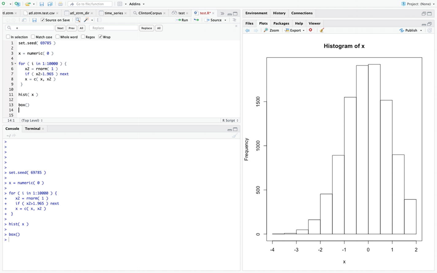
Using a loop to generate a histogram of random standard normal variates that are less then 1.965
Using Indices
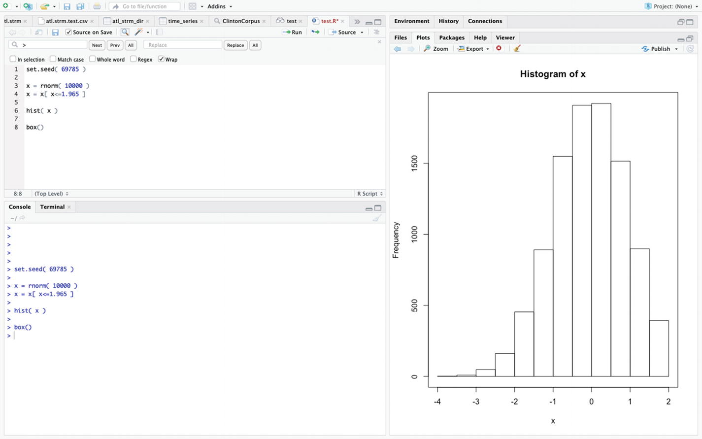
Using indices to generate a histogram of random standard normal variates that are less then 1.965
Note that the two histograms are the same since the seeds are the same and the same 10,000 numbers are used.
If 10,000 is increased to 100,000 above, on my computer the method using loops takes about 34 seconds while the method using indices takes less than 1 second.
A ‘for’ Loop, a ‘repeat’ Loop, an ‘if’ Statement, and a ‘break’ Statement
In this example, random samples of size 100 of standard normal numbers are generated within a repeat loop . The repeat loop is within a for loop that goes through 10,000 iterations.
For each sample, the sum of the sample is divided by the ten and then compared to 1.965. (Since the expected value of the generated numbers is zero, the standard error is one, and the numbers are independent, the sample sum divided by ten is a standard normal variate.) If the value is less than 1.965, then the repeat loop continues. Otherwise, the repeat loop stops, the number of times through the loop is recorded, and the next for loop starts. At the end, the vector of the numbers of times through the loop is plotted in a histogram, and the mean and median of the numbers of times is found.
First, the seed for the random number generator is set. Then, a vector n.hist is created to hold the results, with a place for each iteration of the for loop. Next, the for loop opens, and the counter n is set to zero. Then, the repeat loop opens.
At the beginning of the repeat loop, the counter n is incremented by one. Then, the sample is taken, divided by ten, and summed. The result is set equal to x. Next, the value of x is compared to 1.965 in an if statement. If the value is greater than 1.965, then n.hist for index i is set equal to the counter n and a break statement breaks the function out of the repeat loop. Otherwise, the repeat loop continues looping.
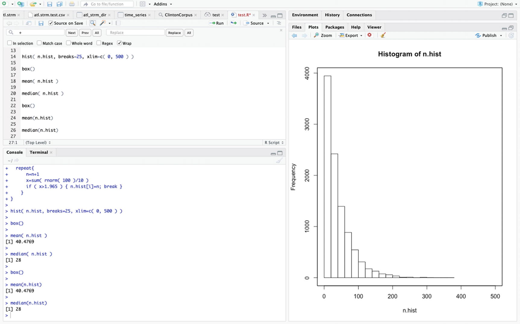
The numbers of times needed until the result exceed 1.965 for sums of 100 standard normal variable divided by 10—using a for loop
Note that the mean is close to 40, which is the expected number of trials necessary on average to see an event with a probability of 0.0247 of occurring. However, the median is much smaller since the distribution is highly skewed.
Using Indices
To do this example using indices, we found the repeat loop necessary, but that the for loop could be dispensed with.
Once again, the random number generator seed is set—to the same number as in the first part of the example—and n.hist is defined numeric with 10,000 elements. Then, the counter n is set to zero, the counter cl.sv is set to zero, and the counter n.col is set to 10,000.
Next, the repeat loop opens. The matrix x is defined as a matrix with 100 rows and n.col columns (initially 10,000). The elements of x are randomly generated standard normal numbers and the number of elements is the product 100 and n.col.
Next, the function apply() is used to sum each column of the matrix, and the result is assigned to x. Then, x is divided by 10. Next, the length of the vector containing those elements of x that are larger than 1.965 is found and assigned to x.
Then, x is added to cl.sv so that cl.sv contains the number of columns for which a result larger than 1.965 has been found. Then, n is incremented by one. Next, x values of n.hist are set equal to n, where cl.sv and x are used to say where along the vector n.hist to put the value of n.
Next, n.col is decremented by the value of x. The repeat loop continues until n.col equals zero. At each iteration, n increases by one.
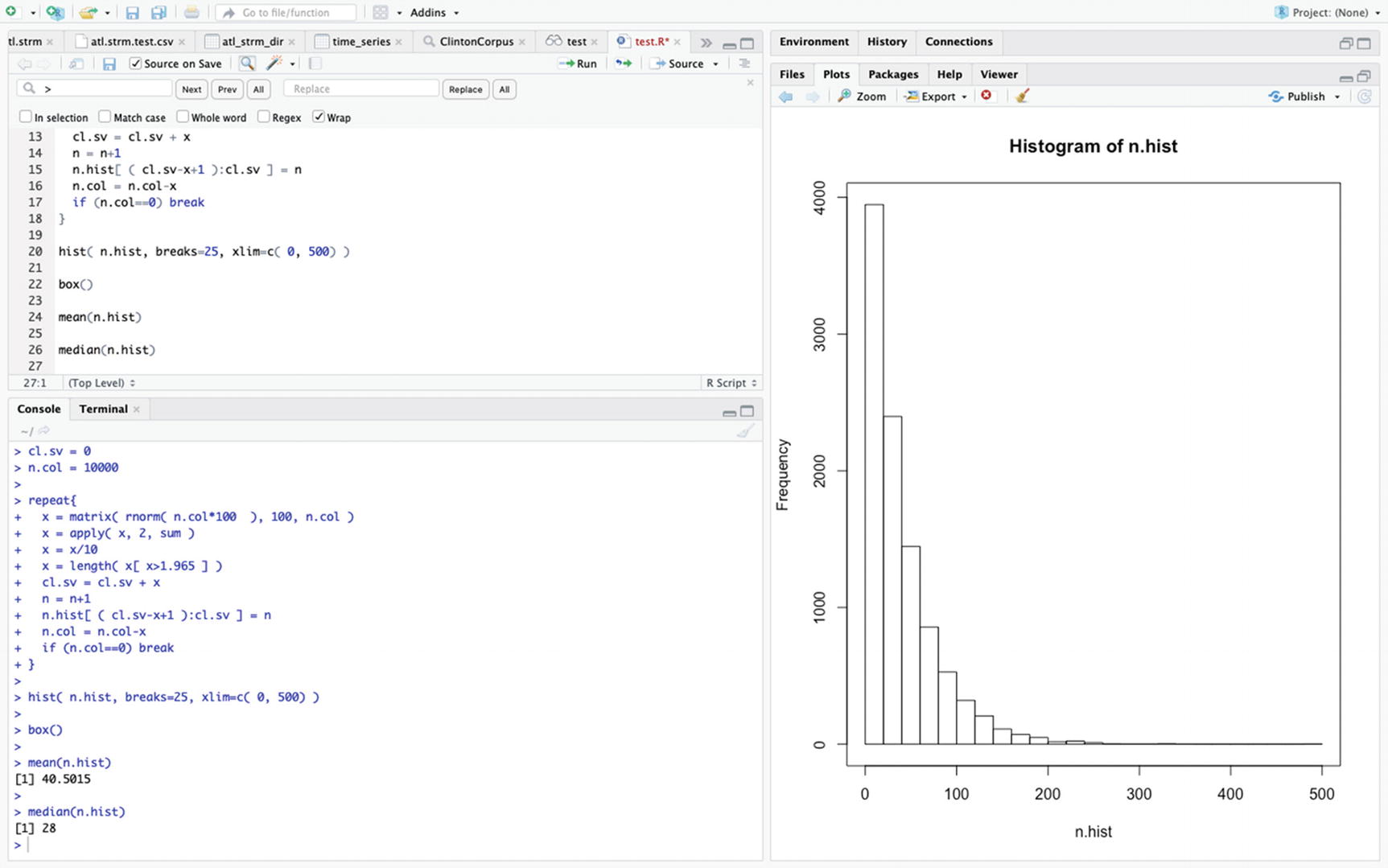
The numbers of times needed to exceed 1.965 for sums of 100 standard normal variable divided by 10—using indices
Once again, the mean is close to 40 and the median is 28.
Both methods use about the same amount of time. If 10,000 is replaced by 100,000 above, then the looping method takes about 44 seconds and the indexing method takes about 45 seconds on my computer.
Since the process of generating the random samples is different between the two methods, the results for the two methods are not identical even though the seed for the random number generator is the same.