
Chapter 5
Scattering from Infinite Cylinders
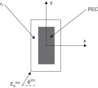
Large radomes are assembled due to fabrication and mechanical considerations from many panels connected together with metallic or dielectric beams, in contrast to small- and medium-sized radomes, which are planar or conformal and made from one piece. The panels are made of thin membranes or sandwiches, which are optimized for minimum transmission loss over the operational frequency band of the radome, as explained in Chapters 2 and 3. The beams introduce scattering effects that degrade the overall electromagnetic performance of the antenna enclosed in the radome, in addition to the transmission losses through the panels. This chapter will describe various numerical methods to compute the scattering effect from a dielectric, conductive and a heterogeneous beam (dielectric beam with conductive strips) with arbitrary cross section, for orthogonal polarizations and for oblique incident angles. The scattering from a beam can be characterized by its scattering pattern and the induced field ratio (IFR) introduced by [1, 2]. The IFR is defined as the ratio of the forward scattered far-field to the hypothetical far-field radiated in the forward direction by a 2D aperture with a width equal to the optical shadow of the beam on the incident wavefront. The IFR depends on polarization, such that IFRe is related to TM incident wave and IFRh is related to TE incident wave. The total scattering effect from an array of beams in front of the enclosed antenna is described in Chapter 6.
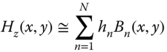
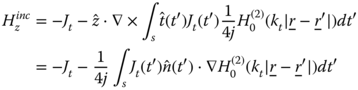
The computation of the scattering from a heterogeneous beam made of dielectric and conductive materials is possible by considering the scattered field as a superposition of the radiation from equivalent electric polarization currents and conductive currents. Evaluation of these equivalent sources can be obtained by formulating two volume-coupled integral equations: the electric field integral equation (EFIE) and the magnetic field integral equation (MFIE). These integral equations are formulated by recognizing that the total field is equal to the summation of the incident field and the scattered field by the beam equivalent electric and magnetic polarization currents. The two integral equations can be solved by the method of moments (MoM) [3] using for this purpose point matching or linear basis functions Bn(x,y). The formulation and the numerical evaluation of the integral equations involved are described in section 5.1.
The volume discretization is necessary to properly model a heterogeneous scatterer and as such is computational intensive. In case of homogeneous or layered geometries, they can be treated with surface integral equation formulation and as such the number of unknowns in the numerical evaluation of the solution can be reduced. In a similar fashion to the volume integral equations, two coupled integral equations EFIE and MFIE are formulated using the equivalence theorem to define equivalent electric and magnetic sources on the beam surface. The formulation of the surface integral equations and their numerical evaluation is described in section 5.2.
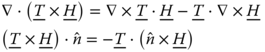
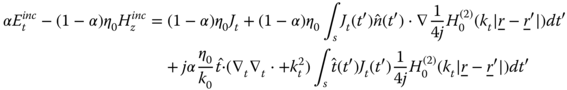
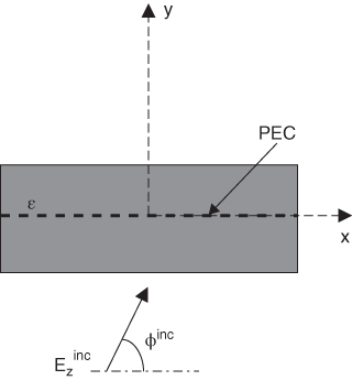
In case of conductive beams, we can use the derivation of the surface integral equation with adaptation to the perfect electric conductor (PEC) boundary conditions ![]() on the beam surface. A further simplification of the surface integral equations is obtained if we recognize that the EFIE and MFIE are uncoupled for orthogonal incident field illumination. This observation simplifies and further reduces the computational complexity of the integral equations solution using the MoM. However, the numerical solution of the integral equations encounters singularity problems, due to internal resonances. These internal cavity resonances are the result of the homogeneous solution of the integral equations and they corrupt the solution at these frequencies. The root of the problem is that the surface integral equation involves only data on the mathematical surface of the scatterer and cannot distinguish between “inside” and “outside” in order to produce the desired external solution. Since the interior resonances are different for the EFIE and MFIE the effect of the interior resonances can be minimized if we combine these integral equations into the so called combined field integral equation (CFIE). The formulation of the surface integral equations and their numerical evaluation is described in section 5.3.
on the beam surface. A further simplification of the surface integral equations is obtained if we recognize that the EFIE and MFIE are uncoupled for orthogonal incident field illumination. This observation simplifies and further reduces the computational complexity of the integral equations solution using the MoM. However, the numerical solution of the integral equations encounters singularity problems, due to internal resonances. These internal cavity resonances are the result of the homogeneous solution of the integral equations and they corrupt the solution at these frequencies. The root of the problem is that the surface integral equation involves only data on the mathematical surface of the scatterer and cannot distinguish between “inside” and “outside” in order to produce the desired external solution. Since the interior resonances are different for the EFIE and MFIE the effect of the interior resonances can be minimized if we combine these integral equations into the so called combined field integral equation (CFIE). The formulation of the surface integral equations and their numerical evaluation is described in section 5.3.
An important objective in the design of space frame radomes made of homogeneous dielectric beams is to reduce the forward scattering of the beams. A possible way to reduce the forward scattering from dielectric beams is to tune them with conductive strips inserted in the dielectric beam volume. The induced currents in the conductive strips offset the effect of the electric polarization currents induced in the homogeneous dielectric beam and reduce the forward scattering of the beam for a limited frequency bandwidth. The analysis of the scattering for these tuned beams is possible by formulating the EFIE of the problem and forcing the tangential electric field along the conductive strips of the beam to be equal to zero. The formulation and the numerical evaluation of scattering from a tuned dielectric beam with vertical and horizontal conductive strips to reduce their forward scattering is described in section 5.4.
Volume integral equation solved by MoM as outlined in section 5.1 is versatile, but involves fully populated matrices and requires relatively large computational effort to treat scatterers of moderate electrical size. On the other hand, surface integral equation matrices are populated as the volume integral equation matrices, but are smaller in size. However, they can accommodate only homogeneous, multilayer, and conductive problems. An alternative option to numerical computation of the scattering from a composite inhomogeneous beam is to solve its differential equation using the finite element method (FEM) [4] and [5]. Comparison of the FEM computational effort to the solution with volume integral equations reveals that it is less computationally intensive, since the matrices involved are sparse, but they are slightly larger in size. The differential equation methods often include an additional region of space outside the scatterer to ensure that the scattered fields represent outward propagating solutions. This additional region must be terminated with a radiation boundary condition, as will be discussed later. The formulation and the numerical evaluation of the scattering from a heterogenous beam using FEM are described in section 5.5.
5.1 Heterogeneous Beams—Volume Integral Equation Formulation
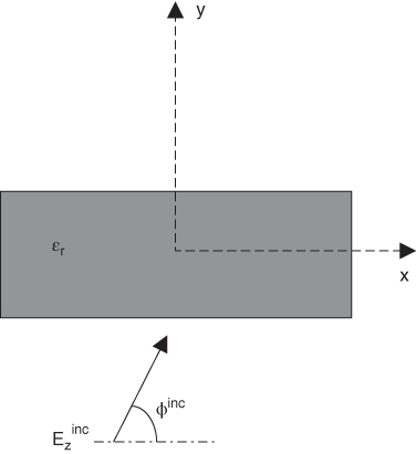
Oblique incidence volume integral equation formulation presented in this section is mainly based on [3]. Other relevant references for normal and oblique TM and TE incidence and volume formulation can be found in [6–10], and [11]. The cross section of the beam is shown in Fig. 5.1. Moreover, the incident field propagation vector components are ![]() and
and ![]() , in which
, in which ![]() , θ0 is the angle between the incident field propagation direction and the beam axis (for normal incidence
, θ0 is the angle between the incident field propagation direction and the beam axis (for normal incidence ![]() ) and ω is the angular frequency.
) and ω is the angular frequency.
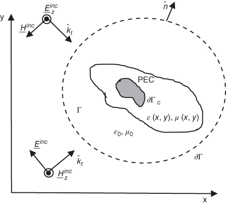
figure 5.1 -Beam geometry.
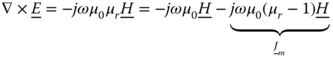
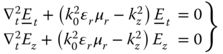
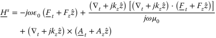
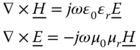
We start with the time harmonic {e jωt} Maxwell equations and introduce equivalent electric ![]() and magnetic currents
and magnetic currents ![]() to represent the polarization currents induced in a medium with relative permittivity ϵr(x,y) and permeability μr(x,y).
to represent the polarization currents induced in a medium with relative permittivity ϵr(x,y) and permeability μr(x,y).
The z dependence of the oblique incident field is ![]() with kz being the propagation constant in z direction and correspondingly, we assume that the z dependence of the total fields in the system is also
with kz being the propagation constant in z direction and correspondingly, we assume that the z dependence of the total fields in the system is also ![]() . Thus, the total electric and magnetic fields can be described by
. Thus, the total electric and magnetic fields can be described by
in which ![]() are the transverse electric and magnetic fields and
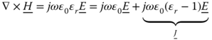
are the transverse electric and magnetic fields and ![]() are the z-components of the electric and magnetic fields. Suppose that the cylinder cross section is modeled by triangular cells of constant permittivity and permeability, but varying from cell to cell. The total scattering from the beam would be the superposition of the scattering from all these various homogeneous triangular cells. Let's define the operators
are the z-components of the electric and magnetic fields. Suppose that the cylinder cross section is modeled by triangular cells of constant permittivity and permeability, but varying from cell to cell. The total scattering from the beam would be the superposition of the scattering from all these various homogeneous triangular cells. Let's define the operators ![]() and
and ![]() to obtain the differential equations for the magnetic field of each triangular cell:
to obtain the differential equations for the magnetic field of each triangular cell:
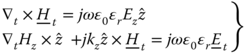
Similarly, we obtain for the electric field
Substitution of (5.5) and (5.6) into (5.1)–(5.4) yields
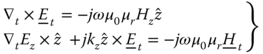
Moreover, if we apply the operator ![]() on (5.9) and substitute (5.7), we obtain after some algebraic manipulations,
on (5.9) and substitute (5.7), we obtain after some algebraic manipulations,
We can define the transverse and longitudinal equivalent polarization magnetic currents ![]() , Jmz and express them in terms of the z-directed electric and magnetic components of the fields.
, Jmz and express them in terms of the z-directed electric and magnetic components of the fields.
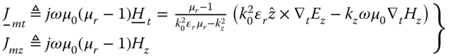
Similarly, one can show that
and the transverse and longitudinal electric polarization currents ![]() and Jz are,
and Jz are,
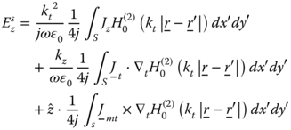
The equivalent polarization currents radiate in free space, but are unknown quantities since they depend on the total field components Ez and Hz. If we denote by ![]() the electric and magnetic fields due to the electric currents and the fields
the electric and magnetic fields due to the electric currents and the fields ![]() due to the magnetic currents by superposition we can rewrite the total fields,
due to the magnetic currents by superposition we can rewrite the total fields,
We define ![]() and
and ![]() in which
in which ![]() is the vector magnetic potential and
is the vector magnetic potential and ![]() is the vector electric potential. Thus, substitution of the vector potentials into Maxwell eqs. (5.1) and (5.2), and using some vector identities yields
is the vector electric potential. Thus, substitution of the vector potentials into Maxwell eqs. (5.1) and (5.2), and using some vector identities yields
in which Φ is the scalar electric potential
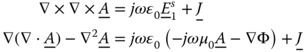
If we use Lorentz gauge ![]() , we obtain
, we obtain
and
Similarly, we obtain the Lorentz gauge for the magnetic currents ![]() with Φm being the magnetic scalar potential and
with Φm being the magnetic scalar potential and
and
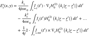
Finally, we get the scattered fields in terms of vector magnetic and electric potentials:
Similarly, for the magnetic field we obtain the expression
Substitution of (5.5) and (5.6) and the explicit expressions of the operators in terms of transverse and longitudinal components into (5.30), yields
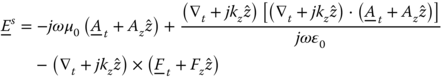
From (5.32), we obtain the explicit form of the z-component
Similarly, for the magnetic scattered field we obtain:
and its associated z-component:

Given a z-directed line source with current ![]() , we can solve the differential equation for Az in cylindrical coordinates (r, φ, z),
, we can solve the differential equation for Az in cylindrical coordinates (r, φ, z),
By symmetry considerations of the line source geometry, we can assume that ![]() . Thus,
. Thus,
and the solution [12] is,
Solution for Jx and Jy yields similar results for ax(r) and ay(r). H0(2)(x) is the second kind Hankel function of zero order. If we repeat the differential equation solution for a magnetic line source current, we obtain the same results but for the electric vector potential components fx(r), fy(r), fz(r). Moreover, displacement of the line source to r' location in (x,y) plane will change the solution to 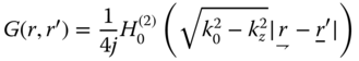 in which
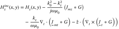
 ![]() . If we extend the derivation to a 2D electric and magnetic current distribution and use superposition for the computation, we obtain the following result for the z-directed electric and magnetic fields,
. If we extend the derivation to a 2D electric and magnetic current distribution and use superposition for the computation, we obtain the following result for the z-directed electric and magnetic fields,
and
in which * denotes convolution. The electric field integral equation (EFIE) and magnetic field integral equation (MFIE) are formulated by recognizing that the total field Ez(x, y) is equal to the summation of the incident field ![]() and the scattered field
and the scattered field ![]() excited by the electric and magnetic polarization currents
excited by the electric and magnetic polarization currents ![]() ,
, ![]() such that
such that

and
in which ![]() and
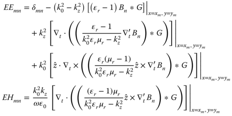
and ![]() with E0 and H0 being the amplitudes of the incident electric and magnetic fields, respectively. These two integral equations can be solved by method of moments (MoM) [3], using, for instance, point matching or linear basis functions Bn(x,y). Thus, the z-component of the electric and magnetic field can be expressed by
with E0 and H0 being the amplitudes of the incident electric and magnetic fields, respectively. These two integral equations can be solved by method of moments (MoM) [3], using, for instance, point matching or linear basis functions Bn(x,y). Thus, the z-component of the electric and magnetic field can be expressed by
and
in which N is the number of basis functions and Bn(x,y) denotes a pyramid basis function centered at the nth corner or node within the triangular-cell model of the cylinder cross section as shown in Fig. 5.2.
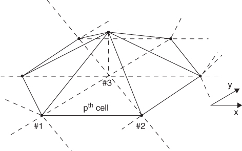
figure 5.2 Linear pyramid basis function.
The basis function connects the triangular cells grouped around a given vertex and vanishes at every other node in the model. Within the pth cell, there are three nodes i = 1,2,3 and the field can be described as
The coefficients a1, a2, and a3 can be evaluated in terms of the field values at the cell vertices c1, c2, and c3 with corresponding coordinates (x1, y1), (x2, y2), (x3, y3) such that
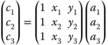
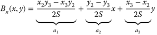
Solution of (5.46) for (a1, a2, a3) yields

with ![]() representing the area of the triangle cell. Accordingly, the basis function as shown in Fig. 5.2 can be derived from (5.45) and (5.47) for c1 = 1, c2 = 0, c3 = 0.
representing the area of the triangle cell. Accordingly, the basis function as shown in Fig. 5.2 can be derived from (5.45) and (5.47) for c1 = 1, c2 = 0, c3 = 0.
Substitution of (5.43), (5.44) into (5.41) and (5.42) and evaluation at discrete points (xm,ym) with m = 1..N in the cylinder cross section yields the matrix equation

in which

Because the z-components of the fields are linear functions within this representation, transverse fields and transverse current densities are constant within a triangular cell. Let us denote
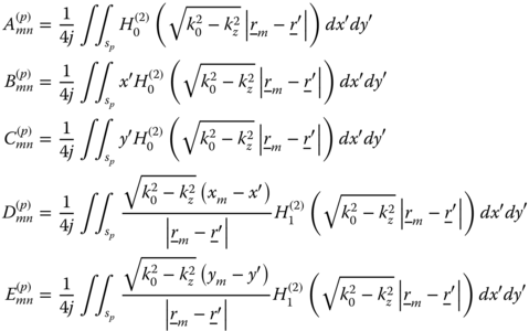
in which sp denotes the area of the pth triangle with a vertex at (xn, yn). H0(2) and H1(2) are the second kind Hankel functions of zero and first order, respectively. The convolutions in (5.54) are two-dimensional integrals. In general, all of the convolution integrals must be evaluated by numerical quadrature. Substitution of (5.48) into (5.50)–(5.53), evaluation of the vector operations, and substitution of (5.54) yields the following:

in which Pn is the total number of triangles with vertex at (xn, yn). Each entry in (5.55)–(5.58) represents a contribution from a source that is distributed over several adjacent triangular cells. The electric and magnetic fields vectors in (5.49) can be evaluated by matrix inversion.
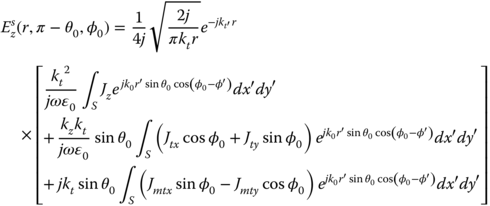
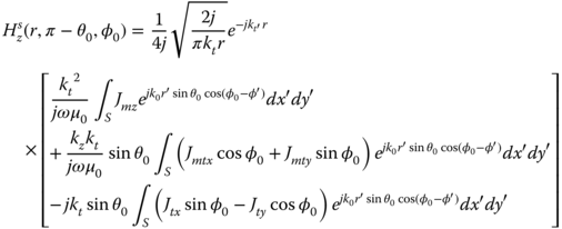
An important parameter, which characterizes the scattering from a beam, is the IFR. The IFR is equal to the ratio of the maximum forward far-field scattering field to the hypothetical forward maximum radiated far field from a 2D aperture with a width equal to the optical projected width of the beam on the incident plane wave front. The aperture field distribution is equal to the incident field [12]. The IFR depends on polarization, such that IFRe is related to TM incident wave and IFRh is related to TE incident wave. Usually, the maximum forward scattering occurs in the propagation direction of the incident wave, as shown in Fig. 5.3, with the maximum forward-scattering direction (θ = π – θ0, φ = φ0).
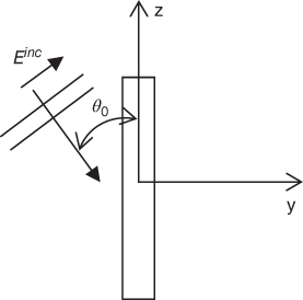
figure 5.3 The geometry of the oblique incident beam.
Eq. (5.39) can be rewritten in the form
in which ![]() and
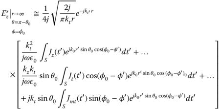
and ![]() . S denotes the cross-section area of the beam and the electric and magnetic current distributions have been computed numerically using the MoM, as explained above. Next, we need to evaluate the scattered field for far-field approximation and use the expressions of Hankel functions for large arguments [13]:
. S denotes the cross-section area of the beam and the electric and magnetic current distributions have been computed numerically using the MoM, as explained above. Next, we need to evaluate the scattered field for far-field approximation and use the expressions of Hankel functions for large arguments [13]:
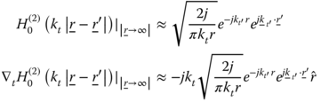
Evaluation of the phase term in (5.60) for ![]() , φ = φ0 yields
, φ = φ0 yields

Evaluation of (5.59) for far field ![]() approximation using (5.60), (5.61) and the representation of
approximation using (5.60), (5.61) and the representation of ![]() in Cartesian coordinates
in Cartesian coordinates ![]() yields
yields
Similar derivation enables to compute the maximum radiated electric field in the direction θ = π – θ0, φ = φ0 by an infinite aperture in z direction with width w positioned at the origin embedded in an infinite conductive plane and illuminated by the same TM polarization oblique incident field as the beam:
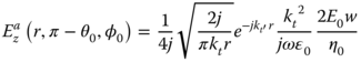
in which ![]() . The ratio of (5.62) and (5.63) results in the expression of IFRe, such that
. The ratio of (5.62) and (5.63) results in the expression of IFRe, such that

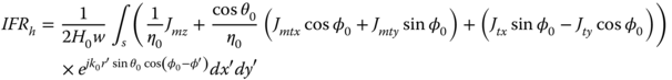
By a similar derivation eq. (5.40) can be rewritten for far field ![]() approximation for the maximum forward scattered magnetic field by,
approximation for the maximum forward scattered magnetic field by,
In a similar fashion, we consider the maximum radiated TE polarized magnetic field in the direction θ = π − θ0, φ = φ0 by an infinite aperture with width w,
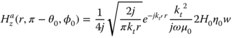
The ratio of (5.65) and (5.66) results in the expression of IFRh, such that
An alternative figure of merit to describe the scattering from the scatterer is the radar cross section (RCS). For TM polarization the RCS is defined by

and for TE polarization,
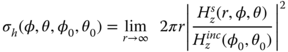
Fig. 5.4 shows the bistatic scattering of a rectangular beam 1.38 × 6.2 in.2 with ϵr = 4.6, tan δ = 0.014 illuminated normally by a plane wave on its narrow side at 5 GHz for TEz and TMz polarizations. The simulation was performed with HFSS commercial software from ANSYS. One can observe a higher scattering of the TEz polarization.

figure 5.4 Bistatic scattering of a rectangular beam 1.38 × 6.2 in.2 with ϵr = 4.6, tan δ = 0.014 normal incidence illumination by a plane wave on its narrow side at 5 GHz for TEz polarization (solid line) and TMz polarization (dash line) simulated with HFSS.
Fig. 5.5 shows the IFR (amplitude and phase) as a function of frequency for two orthogonal polarizations and an incident plane wave on the beam narrow side. The beam is dielectric with mechanical and electrical properties as shown in Fig. 5.4. It is interesting to note that the IFRh is higher and more oscillating compared to IFRe.
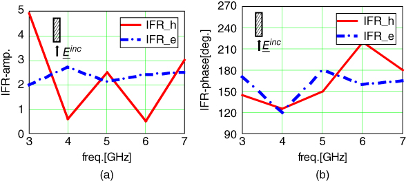
figure 5.5 IFR as function of frequency for a dielectric beam with dimensions 1.38 × 6.2 in.2 with ϵr = 4.6, tan δ = 0.014 and illuminated by a normal plane wave on its narrow side: (a) IFR-amplitude; (b) IFR-phase.
5.2 Homogeneous Beams—Surface Integral Equation Formulation
A volume discretization is necessary to model properly a heterogeneous scatterer and as such is computational intensive. In case of homogeneous, layered geometries, and conductive cylinders, they can be treated with surface integral equation formulation and consequently reduce the required number of unknowns in the MoM numerical algorithm [14]. Therefore, this method is considered as a more efficient alternative to the volume integral equation discussed in the previous section. In the derivation, the equivalence principle [15] is used. Fig. 5.6 shows the beam geometry and the equivalent sources for the external and internal methods.
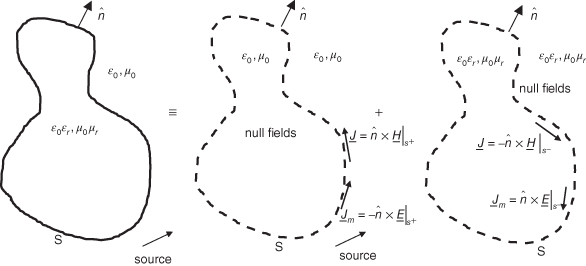
figure 5.6 The homogeneous geometry and its external and internal equivalent problems.
For the EFIE, we consider the tangential electric field at S+ and S- such that
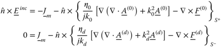
in which ![]() ,
, ![]() and
and ![]() ,
, ![]() are the magnetic and electric vector potentials in free space and in the homogeneous beam, respectively. Similarly, for the MFIE we consider the tangential magnetic field at S+ and S- such that
are the magnetic and electric vector potentials in free space and in the homogeneous beam, respectively. Similarly, for the MFIE we consider the tangential magnetic field at S+ and S- such that

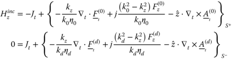
The z dependence of the oblique incident field is ![]() and correspondingly, we assume that the z dependence of the total fields in the system is also
and correspondingly, we assume that the z dependence of the total fields in the system is also ![]() , in which
, in which ![]() . The electric and magnetic fields can be described by (5.5), (5.6) and the incident fields for the TM and TE cases are
. The electric and magnetic fields can be described by (5.5), (5.6) and the incident fields for the TM and TE cases are ![]() and
and ![]() with E0 and H0 being the incident electric and magnetic field intensity, respectively. Let's define the operators
with E0 and H0 being the incident electric and magnetic field intensity, respectively. Let's define the operators ![]() and
and ![]() . Substitution of these operators in (5.70) and (5.71) results in
. Substitution of these operators in (5.70) and (5.71) results in

and
in which

where i = 0,d and ![]() .
. ![]() is the unit vector tangent to the cylinder contour, as shown in Fig. 5.7.
is the unit vector tangent to the cylinder contour, as shown in Fig. 5.7.
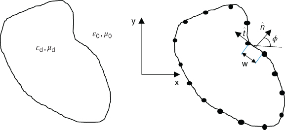
figure 5.7 Flat-strip model of the surface of a homogeneous dielectric cylinder.
Eq. (5.72)a and (5.73)a should be evaluated with the observer an infinitesimal distance outside S, while (5.72)b and (5.73)b should be evaluated with the observer an infinitesimal distance inside S. Equations (5.72) and (5.73) can be solved with MoM with N pulse basis functions on the cylinder contour used to represent the unknowns Jz, Jt, Jmz, Jmt and delta functions as testing functions enforced at the center of each of the cells of the model. The result is a matrix 4 × 4 block structure:

where
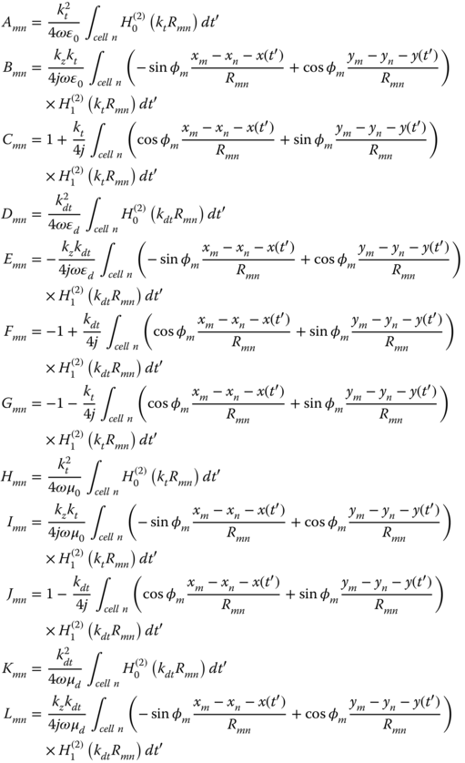
in which  , and φm is the polar angle defining the outward normal vector to the nth strip in the model shown in Fig. 5.7.
In the next step, the IFR of the cylinder can be evaluated. For this task, we need to evaluate the forward-scattered far-field approximation using the expressions of Hankel functions for large arguments [13]. The maximum forward-scattering occurs in the propagation direction of the incident wave, (θ = π – θ0, φ = φ0). In the TM case based on (5.72), the z-directed scattered electric field is
Evaluation of the scattered field for far-field approximation, using the expressions of Hankel functions for large arguments in eq. (5.60) and the phase argument for (θ = π – θ0 φ = φ0) described in eq. (5.78) yields
Derivation of the maximum radiated electric field in the direction θ = π – θ0, φ = π/2 by an infinite aperture with width w, as shown in eq. (5.63) and taking the ratio of (5.79) and (5.63) yields the IFRe for the homogeneous dielectric cylinder,

By similar derivation for the TE case we obtain the forward scattered magnetic field:
and the IFRh is

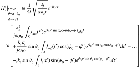
Fig. 5.8 shows the back-scattering RCS from a circular dielectric cylinder with radius a = 24 mm, for normal incidence TM polarized as a function of frequency. The cylinder is a lossy dielectric with ϵr = 4 and σ = 0 (solid line), 0.017 S/m (dot line), 0.05 (dash-dot line) S/m.
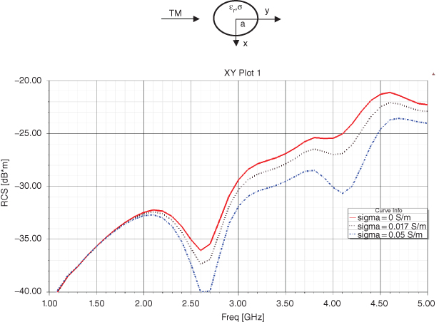
figure 5.8 The back scattering RCS from a circular dielectric cylinder with radius a = 24 mm, for normal incidence TM polarized as a function of frequency. The cylinder is a lossy dielectric with ϵr = 4 and conductivity σ = 0 (solid line), 0.017 S/m (dot line), 0.05 S/m (dash-dot line). All simulations are performed with HFSS.
One can observe that increase in the cylinder conductivity reduces the back scattering.
Fig. 5.9 shows the RCS of a lossless elliptic cylinder (ϵr = 2) with major axis radius a = 38 mm and minor radius axis b = 19 mm illuminated by normal incidence TM polarized wave at angle φinc = 60 deg with respect to x-axis.
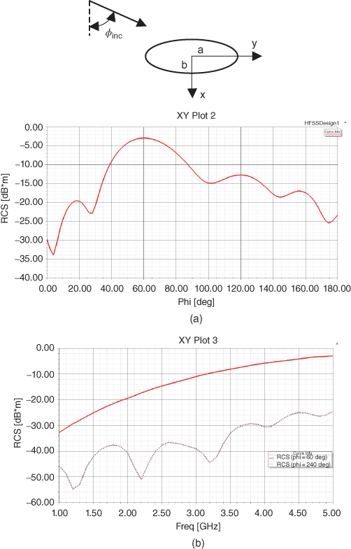
figure 5.9 RCS of lossless elliptic cylinder (ϵr = 2) with a = 38 mm and b = 19 mm illuminated by normal incidence TM polarized wave at angle φinc = 60 deg with respect to x-axis: (a) scattering pattern at 5GHz; (b) forward (φ = 60 deg, solid line) and backward (φ = 240 deg, dot line) RCS as a function of frequency. All simulations are performed with HFSS.
One can observe the forward and backward scattering as a function of frequency in the range 1–5 GHz. In the scattering pattern at 5 GHz, one can observe the forward scattered lobe with peak at φ = 60 deg and a minor lobe in the direction of the specular reflection at φ=120 deg. Fig. 5.10 shows the comparison of the numerical SIE solution (MoM with N = 20 contour divisions) and the exact solution of the TE bistatic RCS of three types of circular cylinders with parameters (ϵr = 1, μr = 10, k0a = 0.7), (ϵr = 9, μr = 5, k0a = 0.7), and (ϵr = 9, μr = 1, k0a = 2).
figure 5.10 Comparison of bistatic RCS between SIE and exact solutions for three penetrable circular cylinders with normal incidence TE excitations [14].
The agreement of the numerical solution with the exact solution is good but slightly inferior to that of the TM polarization, as shown in Fig. 5.8.
5.3 Conductive Beams—Surface Integral Equation Formulation
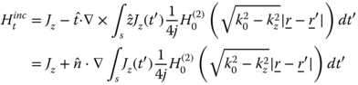
In case of conductive beams, we can use the derivation of the surface integral equation with adaptation to the perfect electric conductor (PEC) boundary conditions ![]() on the beam surface [16]. Thus, for oblique incidence as shown in Fig. 5.3 and TM case, we can consider only the z-directed scattered electric field due to z-directed induced currents and the corresponding EFIE based on (5.72). In this case, no transverse electric and magnetic currents are induced; therefore,
on the beam surface [16]. Thus, for oblique incidence as shown in Fig. 5.3 and TM case, we can consider only the z-directed scattered electric field due to z-directed induced currents and the corresponding EFIE based on (5.72). In this case, no transverse electric and magnetic currents are induced; therefore,
Similarly, based on (5.71)a, one can derive the MFIE. We start with the boundary condition ![]() , which simplifies to
, which simplifies to
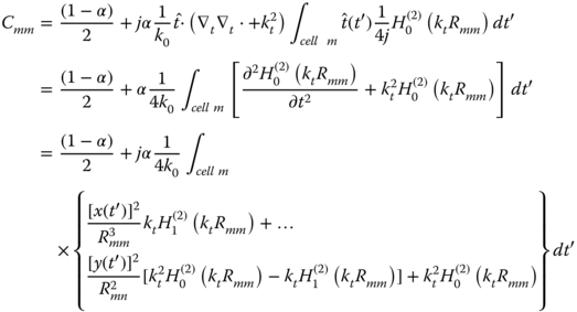
Numerical solution of the integral equations (5.83) and (5.84) encounters singularity problems, due to internal resonances. These internal cavity resonances are the result of the homogeneous solution of the integral equations and they corrupt the solution at these frequencies. The root of the problem is that the surface integral equation involves only data on the mathematical surface of the scatterer and cannot distinguish between “inside” and “outside” in order to produce the desired external solution. Since the interior resonances are different for the EFIE and MFIE, the effect of the interior resonances can be minimized if we combine these integral equations into the so-called combined field integral equation (CFIE) [5]:

In eq. (5.85), we linearly combine eqs. (5.83) and (5.84) using the scale factors α and (1 – α)η0 to employ the same units, where α is a real value between 0 and 1 and η0 is the characteristic impedance of the host medium. However, this CFIE remains valid if ![]() is purely imaginary, which would occur if kz > k. There are no interior resonances frequencies with kz>k, and consequently, the conventional EFIE and MFIE alone would be more efficient choice throughout the invisible region of the spectrum. Eq. (5.85) can be solved numerically using the point matching MoM. The incident field for the TM case is
is purely imaginary, which would occur if kz > k. There are no interior resonances frequencies with kz>k, and consequently, the conventional EFIE and MFIE alone would be more efficient choice throughout the invisible region of the spectrum. Eq. (5.85) can be solved numerically using the point matching MoM. The incident field for the TM case is ![]() and
and ![]() . Using N pulse basis functions and N Dirac testing functions produces the matrix equation
. Using N pulse basis functions and N Dirac testing functions produces the matrix equation

in which j1…jN are the z-directed currents and e1…eN are the z-directed incident fields on the beam contour. Using the convention outlined in Fig. 5.7, the definition of ![]() and
and ![]() in eq. (5.75) and the approximations made for Rmm→0 in (5.77), the diagonal and off-diagonal entries in (5.86) are determined by
in eq. (5.75) and the approximations made for Rmm→0 in (5.77), the diagonal and off-diagonal entries in (5.86) are determined by
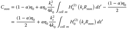
and

in which ![]() and the entries of the excitation column vector are
and the entries of the excitation column vector are
Matrix inversion of (5.87) results in the z-directed currents on the beam contour. The knowledge of the currents enable to compute the IFRe based on (5.80), given that in this case only z-directed electric currents are excited,
where w is the optical projected width of the conductive beam on the incident wave plane and Jz is defined in Fig. 5.3 with the maximum forward-scattering direction (θ = π – θ0, φ = φ0).
Similar derivation can be applied for the TE case. The incident field for the TE case is ![]() and
and ![]() . In this case, we encounter only
. In this case, we encounter only ![]() components of the excited electric current
components of the excited electric current ![]() . The boundary conditions on the beam surface is
. The boundary conditions on the beam surface is  . Substitution of (5.27) for
 ![]() and (5.35) for
and (5.35) for ![]() yields the EFIE; in this case, i.e.,
yields the EFIE; in this case, i.e.,
The MFIE is based on the boundary condition ![]() , which can be simplified using (5.35) to
, which can be simplified using (5.35) to
To avoid the interior resonances excited in the EFIE and MFIE formulations in a similar fashion to the TM case, we linearly combine the two integral equations into the CFIE for the TE case:
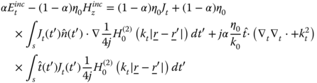
In (5.93) the scale factors α and (1 – α)η0 are used to employ the same units, where α is a real value between 0 and 1 and η0 is the characteristic impedance of the host medium. Eq. (5.93) can be solved numerically using the MoM with N pulse basis functions and N Dirac delta-testing functions to obtain the matrix eq. (5.94):

in which jt1…jtN are the tangential currents on the beam contour and e1…eN are the tangential incident fields on the beam contour. Using the convention outlined in Fig. 5.7, the definition of ![]() and
and ![]() in eq. (5.75) and the approximations made for Rmm→0 in (5.77), the diagonal and off-diagonal entries in (5.94) are determined:
in eq. (5.75) and the approximations made for Rmm→0 in (5.77), the diagonal and off-diagonal entries in (5.94) are determined:
and

in which ![]() and the entries of the excitation column vector are
and the entries of the excitation column vector are
Matrix inversion of (5.94) results in the tangential currents on the beam contour on the beam contour. The knowledge of the currents enables to compute the IFRh based on (5.82) with the maximum forward-scattering direction coinciding with axis (θ = π – θ0, φ = φ0). Given that in this case only transverse electric currents are excited,
where w is the optical projected width of the conductive beam on the incident wave plane and Jt is defined in Fig. 5.3.
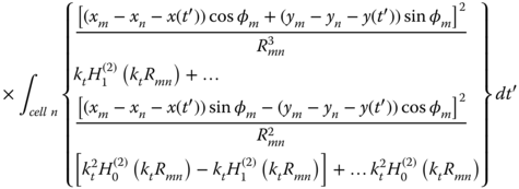
Fig. 5.11 shows the comparison of the numerical solutions of the EFIE, CFIE, and the exact solutions for the TM current density on a circular PEC cylinder of radius 0.82λ0 [5].
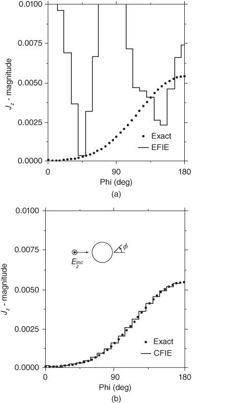
figure 5.11 Comparison of the EFIE, CFIE, and exact solutions for the TM current density on a circular PEC cylinder of radius 0.82λ0. The numerical result was obtained using 40 equal sized cells: (a) EFIE and exact current distribution results; (b) CFIE and exact current distribution results [5].
One can observe the distortion in the current distribution computed with EFIE due to the internal singularities compared to the exact solution. All that is in contrast to the numerical solution using CFIE, in which exists a nice agreement with the exact solution. Fig. 5.12 shows the comparison of the EFIE, CFIE, and exact solutions for the TM bistatic radar cross section scattering patterns from the circular PEC cylinder of radius a = 0.82λ0 [5]. In this case, good agreement is obtained for both numerical solutions (EFIE and CFIE) and the exact solution. This observation implies that the internal singularities affect the current distribution on the scatterer and its near field but almost have no effect on the scattered far field. This can be attributed to the fact that the internal singularities affect the reactive scattered fields of the beam and have almost no effect on the real scattered fields, which determine the scattered far field.
figure 5.12 Comparison of the EFIE, CFIE, and exact solutions for the TM bistatic radar cross section scattering patterns from a circular PEC cylinder of radius a = 0.82λ0 [5].
The exact solution of the normalized scattered far field (r→∞) from a circular PEC cylinder is derived using cylindrical wave functions and is described in [15] by
with its corresponding IFRe given by
where Jn and Hn(2) are the Bessel and outgoing Hankel functions and θ0 is the tilt angle between the incident wavefront and the cylinder axis. Similar derivation using the cylindrical wave functions for the TE case yields

with the IFRh given by
In general, the IFRe is larger in magnitude than IFRh and has a positive phase angle compared to a negative phase angle for the HP. Both IFR's approach the value of –1.0 + j0.0 as the radius increases. IFRh approaches this limit from below and IFRe approaches the limit from above.
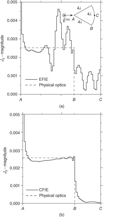
figure 5.13 Comparison of the EFIE, CFIE, and physical optics solutions for the TM current density on a pie-shaped PEC cylinder: (a) EFIE and physical optics distribution results; (b) CFIE and physical optics distribution results [5].
Another example that demonstrates the effect of the internal resonances on the induced current distribution on a pie-shaped PEC cylinder for TM polarization is shown in Fig. 5.13. In a similar fashion to the circular PEC cylinder computation of the current distribution using the CFIE formulation solves the problem almost entirely. In Fig. 5.13 the numerical solution is compared to the induced current computed using physical optics approximation, which is nonzero only on the illuminated surfaces.
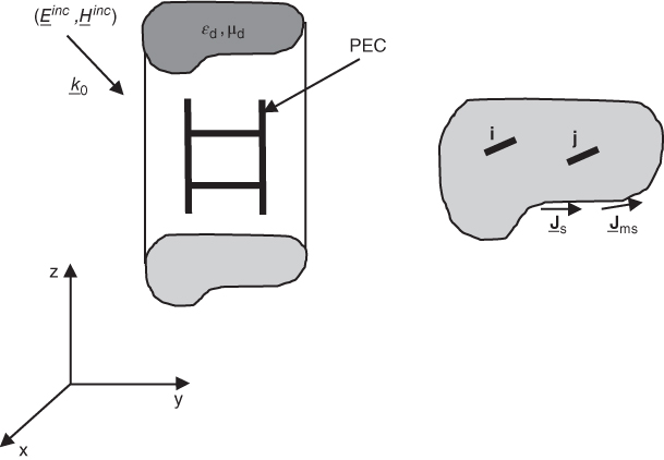
figure 5.14 Tuned-beam geometry with a periodic vertical and horizontal wire loading.
5.4 Tuned Beams—Surface Integral Equation Formulation
The main objective in the design of space frame radomes made of homogeneous dielectric beams is to reduce their forward scattering. This objective can be accomplished by inserting periodic vertical and horizontal conductive strips in the dielectric beam with periodicity Δz in z direction, as shown in Fig. 5.14. Consequently, the strips can be arranged into unit cells and it is sufficient to study the behavior of the electromagnetic field within a single reference unit cell. The induced currents in the conductive strips offset the effect of the electric polarization currents induced in the homogeneous dielectric beam and reduce the forward scattering of the beam for a limited frequency bandwidth. The analysis of the scattering for these tuned beams is possible by formulating the EFIE of the problem by forcing the tangential electric field along the conductive strips of the beam to be equal to zero. Evaluation of the total electric field at the strip locations is done in two steps. In the first step using the coupled surface integral equation of the unloaded homogeneous beam as outlined in Chapter 5.2, the equivalent surface electric currents ![]() and surface magnetic currents
and surface magnetic currents ![]() on the beam contour S, as shown in Fig. 5.6, are evaluated using the MoM using eq. (5.72) for the TM case and eq. (5.73) for the TE case. In the second step, an EFIE is constructed in terms of the unknown induced currents on the conductive strips and enforcing the total electric field on the strips to vanish. The total electric field at the strip locations is equal to the field radiated by the surface equivalent sources on the beam contour S for the unloaded homogeneous beam and the scattered electric fields by the vertical and horizontal conductive strips. The scattered fields by the conductive strips are formulated in terms of a z-directed periodic array of vertical and horizontal current elements
on the beam contour S, as shown in Fig. 5.6, are evaluated using the MoM using eq. (5.72) for the TM case and eq. (5.73) for the TE case. In the second step, an EFIE is constructed in terms of the unknown induced currents on the conductive strips and enforcing the total electric field on the strips to vanish. The total electric field at the strip locations is equal to the field radiated by the surface equivalent sources on the beam contour S for the unloaded homogeneous beam and the scattered electric fields by the vertical and horizontal conductive strips. The scattered fields by the conductive strips are formulated in terms of a z-directed periodic array of vertical and horizontal current elements ![]() as shown in Fig. 5.14.
as shown in Fig. 5.14.
Without loss of generality, we assume that the horizontal wires are y-directed with center coordinates (xr,yr,zr) and the vertical wires are z-directed with center coordinates (xq,yq,zq). The length of the vertical strips in the unit cell is Lv and the length of the horizontal strips is Lh with the strips width being w. The current singularity near the strip edges [17] is taken in consideration for the vertical strips by assuming that the transverse current distribution is  and
and  for the horizontal strips. Accordingly, the z-periodic currents on the conductive strips of the beam can be represented by a Fourier series:
Here, ![]() with n = 0,1,…, denoting the Floquet harmonics [17] index, Δz being the unit cell length in z direction and
with n = 0,1,…, denoting the Floquet harmonics [17] index, Δz being the unit cell length in z direction and ![]() . The center locations of the horizontal strips are (xr,yr,zr) with r = 1,…,R and R being the total number of horizontal strips in the unit cell. The center locations of the vertical strips are (xq,yq,zq) with q = 1,…,Q and Q being the total number of vertical strips in the unit cell. The electric field scattered by this current distribution can be described by
. The center locations of the horizontal strips are (xr,yr,zr) with r = 1,…,R and R being the total number of horizontal strips in the unit cell. The center locations of the vertical strips are (xq,yq,zq) with q = 1,…,Q and Q being the total number of vertical strips in the unit cell. The electric field scattered by this current distribution can be described by
in which ![]() and
and  where
where ![]() ,
, ![]() , and v being the unit cell volume. The EFIE of the problem is set by forcing the tangential components of the total electric field to vanish along the conductive strips. The location along the strips is denoted by rc.
, and v being the unit cell volume. The EFIE of the problem is set by forcing the tangential components of the total electric field to vanish along the conductive strips. The location along the strips is denoted by rc.

in which
where ![]() denotes points on the beam contour. The electric currents,
denotes points on the beam contour. The electric currents, ![]() and magnetic currents,
and magnetic currents, ![]() are the Fourier series of the currents
are the Fourier series of the currents ![]() and
and ![]() evaluated in advance, as explained in section 5.2. The currents
evaluated in advance, as explained in section 5.2. The currents ![]() on the strips can be determined by solving (5.105) using the MoM with pulses as basis functions and delta functions as test functions. The matrix inversion used in the MoM is performed for each harmonics n. Only the zeroth order harmonics (n = 0) is propagating, but few harmonics are needed to evaluate the total field in the beam. The next essential step is evaluation of the scattered far field of the tuned beam. As an interim step, we need to compute the total electric and magnetic field in the beam medium given the beam contour surface currents
on the strips can be determined by solving (5.105) using the MoM with pulses as basis functions and delta functions as test functions. The matrix inversion used in the MoM is performed for each harmonics n. Only the zeroth order harmonics (n = 0) is propagating, but few harmonics are needed to evaluate the total field in the beam. The next essential step is evaluation of the scattered far field of the tuned beam. As an interim step, we need to compute the total electric and magnetic field in the beam medium given the beam contour surface currents ![]() ,
, ![]() and the evaluated conductive strip currents
and the evaluated conductive strip currents ![]() using
using
Using (5.107), the induced equivalent volumetric electric and magnetic currents in the beam volume can be computed using (5.17) and (5.19) to represent the induced polarization currents in the beam. Next, the forward far field can be computed using the induced electric and magnetic polarization currents in the beam and the electric currents on the strips. For this step, only the n = 0 propagating harmonics is needed. Without loss of generality, in the special case of incident field propagating in φ = π/2 direction and maximum forward-scattered electric field also in φ = π/2 direction, we can use (5.107) to compute the far-field approximation and the IFR values using (5.64) and (5.67).
Fig. 5.15 shows the geometry of a rectangular dielectric cylinder (ϵr = 3) loaded periodically with two horizontally and two vertically oriented PEC strips in the unit cell [17] with parameters sv = 0.6, sh = 0.8, and p = 0.75. The widths of the strips are wv = wh = 0.01L.
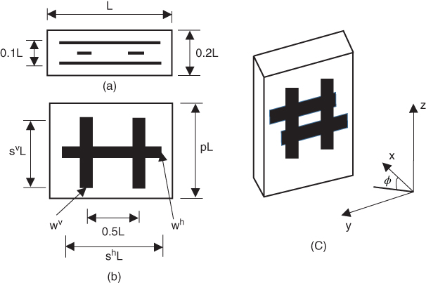
figure 5.15 Rectangular dielectric cylinder, loaded periodically with two horizontally and two vertically oriented PEC strips: (a) cross section: (b) front view; (c) perspective view.
Fig. 5.16 shows the simulated RCS of the loaded and unloaded cylinder as a function of frequency for TE and TM polarizations. One can observe that for normal incidence and TE/TM polarizations, the RCS of the loaded dielectric cylinder is reduced by approximately 30 dB in a narrow frequency bandwidth, with center frequency 2.7 GHz for TE polarization and 3.1 GHz for TM polarization.
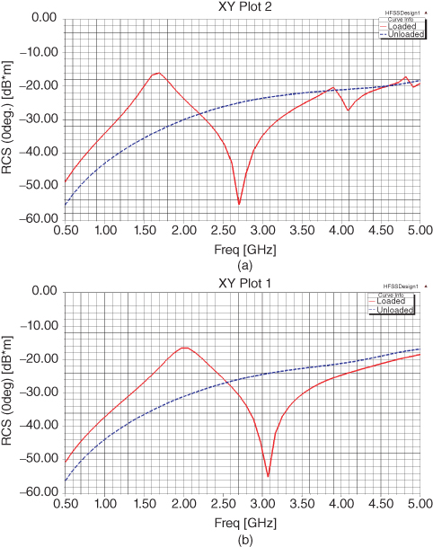
figure 5.16 RCS (0 deg) of the unloaded and loaded cylinder as a function of frequency, for sv = 0.6, sh = 0.8, and p = 0.75: (a) TE polarization; (b) TM polarization. All simulations are performed with HFSS.
In a different example, a rectangular dielectric beam with electrical parameters ϵr = 4.6, tan δ = 0.014, and dimensions 2 × 0.4 in.2 is considered. The beam is tuned with a grid of eight vertical conductive strips located on its center line, spaced 0.277 in. apart and with a strip width of 0.062 in. Fig. 5.17 shows the IFR dependence of the tuned and untuned cylinder on frequency. The data presented is for the TM polarization and normal incidence. The computed and measured data are compared.
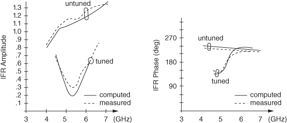
figure 5.17 IFR as a function of frequency for a tuned/untuned dielectric beam 2 × 0.4 in.2 for vertical polarization and normal incidence.
At the tuning frequency of 5.6 GHz, the magnitude of the IFR drops significantly in comparison to that of the untuned beam. In addition, the IFR phase goes through the 180 deg value close to the tuning frequency, a feature common to resonant devices. Fig. 5.18 shows the field distribution (amplitude and phase) of the untuned and tuned beams inside the cross section of the dielectric beam at 5.6 GHz.
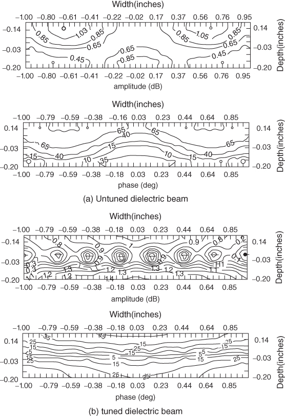
figure 5.18 Field distribution in an untuned and tuned dielectric beam at the tuning frequency (5.6 GHz) at normal incidence: (a) untuned; (b) tuned.
As expected the total electric field goes to zero at the locations of the strips. Moreover, the phase of the electric field is relatively more uniform as compared to that of the untuned beam. The uniformity of the phase distribution is a good indicator of the transparency of the beam because it resembles the uniform phase front of the incident field. Fig. 5.19 shows a comparison between the computed scattering pattern of the untuned and tuned dielectric beams at the tuning frequency of 5.6 GHz.
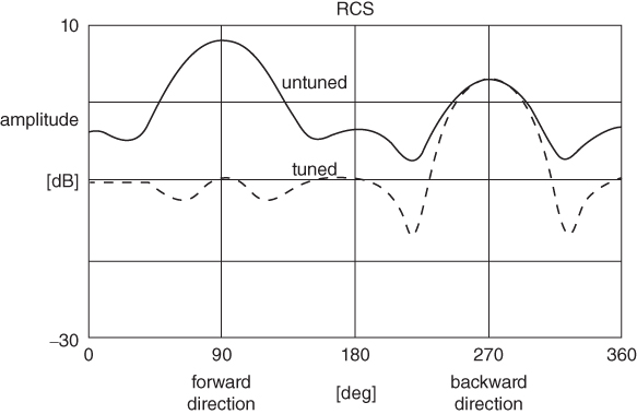
figure 5.19 Scattering pattern for tuned and untuned beam at 5.6 GHz.
One can observe a significant reduction of the scattering levels in the forward direction, as compared to that of the untuned beam.
A different approach to the dual polarization tuning problem (forward scattering reduction) is described in [19]. The concept is based on replacement of soft surfaces by hard surfaces in the dielectric beam for both TEz and TMz polarizations. The presence of hard surfaces on a dielectric or conductive beam is desirable to reduce the beam blockage. Generally, a hard surface supports waves with maximum value of the E-field, like normal electric field on a conductive surface, whereas the soft surface makes the amplitude of the tangential E-field zero at a conductive surface. This effect is not allowing propagation and increases scattering. In case of propagation along a conductive surface, if the E-field excited is normal to the surface it can propagate along the surface with a strong intensity as the boundary condition is hard with ![]() . On the other hand, if the E-field is transverse to the direction of propagation and tangential to the surface, the wave is effectively stopped from propagating along the conductive surface and this increases scattering. Thus, the electric conductor has a strongly polarization dependent boundary condition for waves propagating along it. Accordingly, we are interested to transform the beam surfaces to hard surfaces to reduce scattering. This desire for a dielectric beam for TEz polarization can be obtained by changing the profile of the beam to an oblong shape and strip loading its outer surface with inter-element strip spacing of less than λ/2 to transform the strip periodic structure to a full conductive surface. However, in case we don't have the flexibility to change the cross section of the beam due to mechanical constraints and for instance, still need to reduce the forward scattering of a rectangular cross section dielectric beam, a different approach should be adopted. In this case, two scattering reduction mechanisms are considered, as shown in Fig. 5.20a.
. On the other hand, if the E-field is transverse to the direction of propagation and tangential to the surface, the wave is effectively stopped from propagating along the conductive surface and this increases scattering. Thus, the electric conductor has a strongly polarization dependent boundary condition for waves propagating along it. Accordingly, we are interested to transform the beam surfaces to hard surfaces to reduce scattering. This desire for a dielectric beam for TEz polarization can be obtained by changing the profile of the beam to an oblong shape and strip loading its outer surface with inter-element strip spacing of less than λ/2 to transform the strip periodic structure to a full conductive surface. However, in case we don't have the flexibility to change the cross section of the beam due to mechanical constraints and for instance, still need to reduce the forward scattering of a rectangular cross section dielectric beam, a different approach should be adopted. In this case, two scattering reduction mechanisms are considered, as shown in Fig. 5.20a.

figure 5.20 Measured and calculated blockage widths weq of cylinder realized as parallel-plate waveguide and outer walls of the cylinder coated with strip-loaded dielectric material to obtain the hard boundary condition for both TE and TM cases: (a) geometry; (b) absolute value of weq for TE and TM cases [19].
In the first mechanism, two metal plates are inserted in the dielectric beam to form an internal parallel plate waveguide and the phase propagation through the waveguide is equalized to the phase through air, such that
in which ϵr is the dielectric constant of the beam, k0 is the propagation constant in free space, l is the beam length, and n is an integer. The second tuning mechanism is strip loading of the outer surface with inter-element strip spacing of less than λ/2, which transforms the outer surface to a conductive surface or a hard surface boundary for TEz polarization. The hard surface boundary condition for TMz polarization is obtained by coating the metal plates of the beam by a thin dielectric layer of thickness t, as shown in Fig. 5.20a. Inside the dielectric coating, the propagation constant will be ![]() , which is larger than the k0 outside the coating. The component of kx along the dielectric surface must be equal to k0. Therefore, we will get a normal component of the propagation vector, ky inside the dielectric coating equal to
, which is larger than the k0 outside the coating. The component of kx along the dielectric surface must be equal to k0. Therefore, we will get a normal component of the propagation vector, ky inside the dielectric coating equal to ![]() . This component of kd will transform the boundary condition at the metal surface to the boundary condition of an artificial magnetic conductor at the surface of the dielectric provided that,
. This component of kd will transform the boundary condition at the metal surface to the boundary condition of an artificial magnetic conductor at the surface of the dielectric provided that,
Fig. 5.20b shows the absolute value of ![]() as a function of frequency. One can observe that for the tuned beam with dimensions and parameters outlined in Fig. 5.20a, a minimum in weq, which is proportional to the forward scattering, is obtained at 11.5 GHz.
as a function of frequency. One can observe that for the tuned beam with dimensions and parameters outlined in Fig. 5.20a, a minimum in weq, which is proportional to the forward scattering, is obtained at 11.5 GHz.
Comparison of the two tuning techniques described above reveals that they both can achieve dual polarization forward-scattering reduction in a limited frequency band, but the tuning with vertical and horizontal conductive strips is more flexible from the manufacturing point of view, without the need to use special dielectric materials given a predetermined beam geometry, as may be required based on eqs. (5.108) and (5.109).
5.5 Scattering from Infinite Cylinders—Differential Equation Formulation
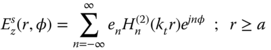
Volume integral equation solved by MoM as outlined in previous sections are versatile, but involve fully populated matrices and require relatively large computational effort to treat scatterers of moderate electrical size. On the other hand, surface integral equation matrices are populated as the volume integral equation matrices, but are smaller in size. However, they can accommodate only homogeneous, multilayer, and conductive problems. An alternative option to compute numerically the scattering from a composite inhomogeneous beam is to solve its differential equation using the finite element method (FEM) [4] and [5]. Comparison of the FEM computational effort to the solution with volume integral equations reveals that it is less computationally intensive, since the matrices involved are sparse, but they are slightly larger in size. The differential equation methods often include an additional region of space outside the scatterer to ensure that the scattered fields represent outward propagating solutions. This additional region must be terminated with a radiation boundary condition as will be discussed later. Fig. 5.21 shows the cylinder geometry confined to the volume Γ made of a composite material with permittivity ϵr(x,y), permeability μr(x,y) and PEC conductive surfaces denoted by ∂Γc. The surface that confines the computational domain is ∂Γ.
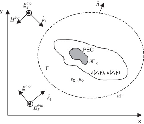
figure 5.21 Cross section of the cylinder geometry showing the imbedded PEC region whose surface is denoted  .
.
In the following, we will consider the general case of oblique scattering as discussed for the integral equation solution and described in [5]. The z dependence of the oblique incident field is ![]() and, correspondingly, we assume that the z dependence of the total fields in the system is also
and, correspondingly, we assume that the z dependence of the total fields in the system is also ![]() . In a similar fashion to the volume integral equation, the electric and magnetic fields in the system can be described by eqs. (5.5) and (5.6). Moreover, we assume that the cylinder cross section is modeled by triangular cells of constant permittivity and permeability, but varying from cell to cell. Then, the total scattering from the beam would be the superposition of the scattering from all these various homogeneous triangular cells. Furthermore, like in the case of the volume integral equation derivation, we employ the total fields Ez and Hz as the primary unknowns to be determined and obtain the transverse magnetic and electric field components within a homogeneous triangular cell via equations (5.16) and (5.18), respectively.
. In a similar fashion to the volume integral equation, the electric and magnetic fields in the system can be described by eqs. (5.5) and (5.6). Moreover, we assume that the cylinder cross section is modeled by triangular cells of constant permittivity and permeability, but varying from cell to cell. Then, the total scattering from the beam would be the superposition of the scattering from all these various homogeneous triangular cells. Furthermore, like in the case of the volume integral equation derivation, we employ the total fields Ez and Hz as the primary unknowns to be determined and obtain the transverse magnetic and electric field components within a homogeneous triangular cell via equations (5.16) and (5.18), respectively.
The electromagnetic fields generated in the vicinity of the scatterer can be determined by the Helmholtz equations for the TM case:
and similarly, for the TE case
Eqs. (5.110) and (5.111) illustrate the “strong” form of Helmholtz equations with the unknown being in a second-order differential operator, which are very sensitive to numerical solution. To make these equations numerically more stable, they can be converted into the so-called “weak” form. The fields in the vicinity of the scatterer must satisfy Maxwell's equations:
Multiplying both sides of (5.112) with the testing function ![]() and integrating over the domain Γ, we obtain
and integrating over the domain Γ, we obtain
Now, recall the two-dimensional divergence theorem
with ![]() being the normal to the surfaces
being the normal to the surfaces ![]() and
and ![]() and the vector identities
and the vector identities
Substitution of (5.114) and (5.115) into (5.113) enables us to rewrite it in the form,
The nabla operator can be rewritten in the form ![]() with
with ![]() . Substitution of the transverse fields from equations (5.16) and (5.18) into (5.116) and utilizing the vector identity
. Substitution of the transverse fields from equations (5.16) and (5.18) into (5.116) and utilizing the vector identity ![]() yields, after some algebraic manipulations,
yields, after some algebraic manipulations,
and

Eqs. (5.117) and (5.118) constitute coupled “weak” differential equations describing the field throughout region Γ and is at the basis of the FEM. For normal incidence kz = 0, we obtain two uncoupled equations one for the TM case (5.117) and the other for the TE case (5.118). Since the tangential electric field must vanish on the conductive surface, Ez is a known function on ![]() and satisfies the Dirichlet boundary condition. Consequently, all testing functions used to discretize (5.118) will vanish on
and satisfies the Dirichlet boundary condition. Consequently, all testing functions used to discretize (5.118) will vanish on ![]() , and the boundary integral will contribute nothing to the matrix equation. Similarly, in the boundary integral
, and the boundary integral will contribute nothing to the matrix equation. Similarly, in the boundary integral ![]() of eq. (5.116), Newman boundary condition is enforced by ignoring the integral over
of eq. (5.116), Newman boundary condition is enforced by ignoring the integral over ![]() . In order to represent the complete scattering problem, it is necessary to augment these equations with additional information about the fields on
. In order to represent the complete scattering problem, it is necessary to augment these equations with additional information about the fields on ![]() , such as radiation boundary conditions (RBC), which will be explained in the following.
, such as radiation boundary conditions (RBC), which will be explained in the following.
For simplicity, we assume that the boundary ![]() is circular with radius a,
is circular with radius a, ![]() and is located in free space. These assumptions simplify the right-hand side (RHS) of (5.117) and (5.118) such that
and is located in free space. These assumptions simplify the right-hand side (RHS) of (5.117) and (5.118) such that

and similarly,
in which ![]() . To comply with the radiation boundary conditions on
. To comply with the radiation boundary conditions on ![]() , the total electric and magnetic fields are expressed as a summation of the scattered fields Ezs, Hzs and the incident fields Ezinc, Hzinc. The scattered electric field on a circular boundary of radius r = a can be expressed in terms of cylindrical harmonics [15] by
, the total electric and magnetic fields are expressed as a summation of the scattered fields Ezs, Hzs and the incident fields Ezinc, Hzinc. The scattered electric field on a circular boundary of radius r = a can be expressed in terms of cylindrical harmonics [15] by
where

and Hn(2)(x) is the nth order Hankel function of second type. Accordingly,

Similarly, the plane wave incident field can be expressed in terms of cylindrical harmonics [15]

where Jn(x) is the nth order Bessel function and
By a similar procedure to that of the scattered field as described in (5.123), we obtain for the incident field

Using the Wronskian relationship [15]:
and addition of (5.123) with (5.126), yields

Similar derivation for Hz, results in
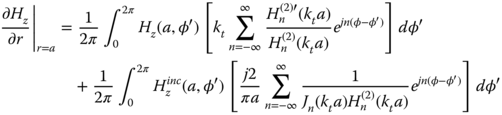
Next we derive ![]() from (5.121) and (5.122)
from (5.121) and (5.122)
and similarly, we obtain

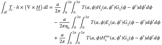
Substituting (5.128)–(5.131) into (5.119) yields the RBC for circular boundary with radius a:
in which ![]() and
and
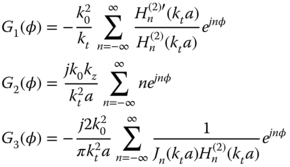
Similarly, (5.120) can be rewritten in the form
Although the summations in (5.133)a and (5.133)b are divergent, the required calculations in (5.132) and (5.134) are well behaved on ![]() , since the integrals involved and the cylindrical harmonic content of the functions Ez(φ) and Hz(φ) ensures that the integrals are convergent and relatively easy to compute. To ensure the convergence, the integration should be performed term by term before the summation. Eqs. (5.132) and (5.134) should be substituted into (5.117) and (5.118) to complete the formulation. The resulting equations can be discretized following the FEM procedure using a piecewise-linear representation Bn(x,y) for Ez(φ) and Hz(φ) and piecewise-linear testing functions Bm(x,y), as shown in Fig. 5.2 and described in eq. (5.48). Each basis function has unity amplitude at one node and vanishes at all other nodes in the mesh. Three basis functions overlap each triangular cell to provide a continuous piecewise-linear representation. Along the circular boundary
, since the integrals involved and the cylindrical harmonic content of the functions Ez(φ) and Hz(φ) ensures that the integrals are convergent and relatively easy to compute. To ensure the convergence, the integration should be performed term by term before the summation. Eqs. (5.132) and (5.134) should be substituted into (5.117) and (5.118) to complete the formulation. The resulting equations can be discretized following the FEM procedure using a piecewise-linear representation Bn(x,y) for Ez(φ) and Hz(φ) and piecewise-linear testing functions Bm(x,y), as shown in Fig. 5.2 and described in eq. (5.48). Each basis function has unity amplitude at one node and vanishes at all other nodes in the mesh. Three basis functions overlap each triangular cell to provide a continuous piecewise-linear representation. Along the circular boundary ![]() the basis and testing functions, Bm(φ) may be expressed as
the basis and testing functions, Bm(φ) may be expressed as
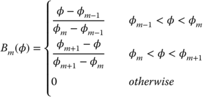
where for convenience, the φ coordinates of the three nodes associated with the mth basis function are denoted as φm-1, φm, and φm+1. The incident uniform plane wave field with amplitude e0 and at an angle (φ0,θ0) on a circular boundary of radius r = a and in terms of cylindrical harmonics can be expressed in terms of
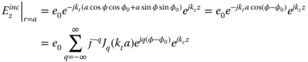
Similarly,

Substitution of (5.43), (5.44), (5.132), (5.134), (5.136), and (5.137) into (5.117) and (5.118) results in the N × N matrix equation with N being the number of nodes in the solution domain:
in which
where
which only contributes to the preceding expressions if node m is located on the circular boundary ![]() . In addition, the excitation vector is given by
. In addition, the excitation vector is given by

Matrix inversion of (5.138) enables to evaluate the electric and magnetic field distributions (e1, e2,….eN) and (h1, h2,…,hN) in the beam. The equivalent induced electric and magnetic polarization currents can be computed using (5.17) and (5.19). Next, the scattered far field and IFRe and IFRh can be computed using (5.64) and (5.67).
Fig. 5.22 shows a comparison of the Ez field produced on the surface of a circular dielectric cylinder with ![]() and ϵr = 50 – j20 by a TE wave incident at an oblique angle of 30 deg computed analytically, numerically with volume integral equation (VIE) and with partial differential equation (PDE) or FEM [20]. The agreement between the analytical and numerical results is very good and also between the VIE and FEM solutions.
and ϵr = 50 – j20 by a TE wave incident at an oblique angle of 30 deg computed analytically, numerically with volume integral equation (VIE) and with partial differential equation (PDE) or FEM [20]. The agreement between the analytical and numerical results is very good and also between the VIE and FEM solutions.

figure 5.22 Comparison of the Ez field produced on the surface of a circular dielectric cylinder with  and ϵr = 50 – j20 by a TE wave incident at an oblique angle of 30 deg computed analytically, numerically with volume integral equation (VIE) and with partial differential equation (PDE) or FEM [20].
References
- 1 Kay, AF. Electrical design of metal space frame radomes. IEEE Trans. Antennas Propagat.,13(2), 188–202, 1965.
- 2 Kennedy, PD. An analysis of the electrical characteristics of structurally supported radomes. The Ohio State University, Columbus, 1958.
- 3 Michielssen, E, Peterson, AF, and Mittra, R. Oblique scattering from inhomogeneous cylinders using a coupled integral formulation with triangular cells. IEEE Trans. Antennas Propagat., 39(4), 485–490, 1991.
- 4 Wu, RB, and Chen, CH. Variational Reaction Formulation of Scattering Problem for Anisotropic Dielectric Cylinders. IEEE Trans. Antennas Propagat., 34(5), 640–645, 1986.
- 5 Peterson, AF, Ray, SL, and Mittra, R. Computational methods for electromagnetics. New York: IEEE Press, 1998.
- 6 Richmond, JH. TE-wave scattering by a dielectric cylinder of arbitrary cross-section shape. IEEE Trans. Antennas Propagat., 14(4), 460–464, 1966.
- 7 Richmond, JH. Scattering by a dielectric cylinder of arbitrary cross section shape. IEEE Trans. Antennas Propagat., 13(3), 334–341, 1965.
- 8 Peterson, AF, and Klock, PW. An improved MFIE formulation for TE-wave scattering from Lossy, inhomogeneous dielectric cylinders. IEEE Trans. Antennas Propagat., 36(1), 45–49, 1988.
- 9 Ricoy, MA, Kilberg, SM, and Volakis, JL. Simple integral equations for two-dimensional scattering with further reduction in unknowns. IEE Proceedings, 136(4), 298–304, 1989.
- 10 Rojas, RG. Scattering by an inhomogeneous dielectric/ferrite cylinder of arbitrary cross-section shape-oblique incidence case,” IEEE Trans. Antennas Propagat., 36(2), 238–246, 1988.
- 11 Gupta, IJ, Lai, AKY, and Burnside, WD. Scattering by dielectric straps with potential application as target support structure. IEEE Trans. Antennas Propagat., 37(9), 1164–1171, 1989.
- 12 Rusch, WVT, Appel-Hansen, J, Klein, CA, and Mittra, R. Forward scattering from square cylinders in the resonance region with application to aperture blockage. IEEE Trans. Antennas Propagat., 24(2), 182–189, 1976.
- 13 Abramowitz, M, and Stegun, IA. Handbook of mathematical functions. New York: Dover, 1964.
- 14 Wu, TK, and Tsai, LL. Scattering by arbitrarily cross-sectioned layered lossy dielectric cylinders. IEEE Trans. Antennas Propagat., 25(4), 518–524, 1977.
- 15 Harrington, RF. Time-harmonic electromagnetic fields. New York: McGraw-Hill, 1961.
- 16 Harrington, RF. Field computation by moment methods. New York: IEEE Press, 1968.
- 17 Michielssen, E, and Mittra, R. Electromagnetic scattering from arbitrary strip loaded cylinders. In IEEE Ant. Propagat. Symposium, Chicago, Illinois, 1992.
- 18 Shavit, R, Smolski, AP, Michielssen, E, and Mittra, R. Scattering analysis of high performance large sandwich radomes. IEEE Trans. Antennas Propagat., 40(2), 126–133, 1992.
- 19 Kildal, PS, Kishk, AA, and Tengs, A. Reduction of forward scattering from cylindrical objects using hard surfaces. IEEE Trans. Antennas Propagat., 44(11), 1509–1520, 1996.
- 20 Peterson, AF. Application of volume discretization methods to oblique scattering from high-contrast penetrable cylinders. IEEE Trans. Mic. Theory Tech., 42(4), 686–689, 1994.
Problems
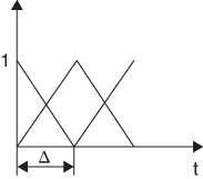
P5.1 A rectangular PEC beam with cross section 1 × 4 in.2 is illuminated by a TMz plane wave with amplitude 1V/m at 60 deg azimuth angle, as shown in the sketch. The operational frequency is 10 GHz.

- a. Write the problem characteristic EFIE with the unknown current distribution on the beam.
- b. Formulate the numerical solution using MoM (point matching). Compute and plot the current distribution on the beam for subdivisions Δ = λ/10, λ/30.
- c. Compute and plot the beam RCS σTM(φ) for subdivisions Δ = λ/10, λ/30.
- d. Repeat items (a) – (c) for TEz incident plane wave and formulation through a MFIE.
- e. Repeat items (a) – (c) for TMz incident plane wave using Galerkin MoM with linear basis functions as shown in the sketch:
Compare solution to that obtained using MoM point matching. Discuss the results and differences.
P5.2 A rectangular PEC beam infinite in z-direction is covered on all its sides by a dielectric layer with thickness 1 cm and dielectric constant ϵr = 4. The cross section of the PEC beam is 1 × 4 in.2 and it is illuminated by a plane wave TMz polarized propagating along y-axis at 10 GHz and with amplitude 1 V/m as shown in the sketch
- a. Write the EFIE integral equation characterizing the problem.
- b. Formulate the numerical solution using point matching MoM volume version. Compute and plot the current distribution on the conductive beam for segmentation Δx × Δy =(λ/10)2, (λ/30)2.
- c. Compute and plot the RCS σTM(φ) for subdivisions Δx × Δy = (λ/10)2, (λ/30)2.
- d. Find the optimal dielectric layer thickness for minimum RCS σTM(π/2).
P5.3 A rectangular PEC beam with cross section 3 × 8 in.2 is illuminated by a TMz plane wave with amplitude 1V/m at 90 deg azimuth angle, as shown P5.1. The operational frequency is 10 GHz.
- a. Formulate the CFIE integral equation with the z-directed unknown current distribution on the beam. Assume coupling coefficient α = 0.2.
- b. Formulate the numerical solution using MoM (point matching). Compute and plot the current distribution on the beam for subdivisions Δ = λ/30.
- c. Compute and plot the scattering pattern from the beam.
- d. Compute and plot the IFRe as a function of w/λ in the range [0.3–4.0] with w being the narrow width of the beam.
P5.4 Repeat problem P5.3 for TEz polarization.
- a. Prove that the CFIE integral equation characterizing the problem is
- b. Formulate the numerical solution of the MFIE and CFIE (with α = 0.2) equations using point-matching MoM and use the conjugate gradient iterative method for matrix inversion.
- c. Compute and plot the current distribution induced on the beam for Δ= λ/20 segmentation.
- d. Compute and plot the RCS σTE(φ) for both formulations MFIE and CFIE. Discuss differences.
- a. Prove that the CFIE integral equation characterizing the problem is
P5.5 Consider a dielectric rectangular beam with dimensions 2 × 0.4 in.2 and dielectric constant ϵr = 4.6, as shown in the sketch:
The beam is illuminated by a plane wave with amplitude 1V/m, at 5.6 GHz, TM polarized and propagating in the direction φinc = 90 deg.
- a. Formulate the EFIE integral eq. of the problem.
- b. Formulate the numerical solution of the EFIE equation using point-matching MoM (volume formulation). Compute and plot the RCS σTM(φ) for cross section segmentation Δx × Δy = (λ/20)2.
On the beam axis, (y = 0) 8 PEC strips were inserted with width 0.062 in. and spacing 0.277 in. between centers, as shown in the sketch:
- c. Formulate the new EFIE equation characterizing the problem.
- d. Formulate the numerical solution using point-matching MoM (volume formulation). Compute and plot the RCS σTM(φ) for cross section segmentation Δx × Δy = (λ/20)2. Assume on the metal strips one basis function. Compare and discuss the results to (b) results.