8 Optimum Linear Systems:
The Kalman Approach
8.1 INTRODUCTION
In the previous chapter optimal linear systems were obtained from the classical Wiener framework to perform operations of filtering prediction and smoothing. The optimal filter was determined in terms of various cross-correlation and autocorrelation functions, or equivalently cross and auto spectral densities, and thus can be considered primarily a frequency domain approach. The Weiner results presented were primarily for wide sense stationary processes; however, for nonstationary processes integral equations were obtained for the solutions. For the case of vector process estimation, the spectral factorization problem for the estimation of wide sense stationary processes proved to be mathematically intractable, and for estimation of nonstationary processes, the resulting integral equations could not be solved by the standard Laplace transform techniques and their solutions were virtually impossible to obtain.
The Kalman filter addresses both the problem of nonstationarity and vector estimation, and it gives the solution in the time domain by virtue of formulating the problem in the state space. Thus rather than the autocorrelation functions or power spectral densities being given, the required information for the Kalman filter solution is given in the state variable format. This information is provided in terms of the state transition, excitation, and measurement matrices of the given state space formulation. This chapter begins with a brief review of discrete time systems and progresses through the description of the various algorithms that are collectively called the Kalman filter. It will also be shown that under steady state conditions, the Kalman and Wiener filters are equivalent for the wide sense stationary case.
In this chapter lowercase letters in the latter part of the alphabet, although not bolded, will indicate vectors. This is because almost all signals indicated will be time-varying vectors or matrices, so bolding the letter would be very distractive. Capital Greek letters will indicate matrices. No distinction will be made between random vectors and deterministic ones because of cumbersomeness of using capital letters; however, for the most part, vectors will be random. Also the traditional square brackets [ ] used in digital signal processing to indicate discrete time signals will be replaced by ( ) where the arguments used are lowercase letters in the middle of the alphabet like j, k, l, m, or n.
8.2 DISCRETE TIME SYSTEMS
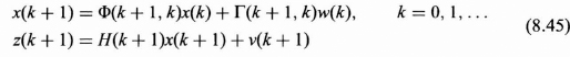
A discrete time linear system with vector input or excitation vector w(k) and output y(k) can be globally illustrated as in Figure 8.1. The system can be further described internally in terms of two equations, called the state equation and output equation:
State Equation:
![]()
Output Equation:
![]()
In these two equations, the following definitions are used:
x(k) is an n × 1 vector called the state vector at time k.
Φ(k + 1, k) is an n × n matrix called the state transition matrix from time k to time k + 1.
Γ(k + 1, k) is an n × p matrix called the excitation transition matrix from time k to time k + 1.
w(k) is a p × 1 vector called the excitation vector at time k.
x(0) is an n × 1 vector called the initial condition or initial state vector at time k = 0.
H(k) is an m × n matrix called the output transition matrix at time k.
y(k + 1) is an m × 1 vector called the output vector at time k + 1.
Equation (8.1a) gives a recursive formula for calculating the state of the system at time index k + 1 as a function of the state of the system at time index k and the excitation vector at time index k. A vector block diagram is shown in Figure 8.2, which illustrates the linear operations on the state and excitation vectors that produce the next state vector.
The solid line indicates a vector operation, and the blocks represent premultiplication by a matrix, the circles a summation of vector components, and the delay represents a one sample delay in time of each component.
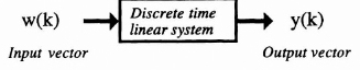
Figure 8.1 Input–output representation of a discrete-time linear system.
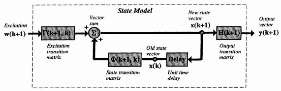
Figure 8.2 Vector block diagram showing the next state and output equations of a discrete-time linear system.
The state x(k) of the system at time k can be obtained in a nonrecursive fashion by solving Eq. (8.1a) for x(k). This solution will be obtained by sequential evaluating x(k). For example, evaluating (8.1a) at k = 0 allows us to solve for x(1) as
![]()
Similarly at k = 1 we have
![]()
Substituting x(1) given before in the equation above, we see that
![]()
Now substituting the x(2) above into Eqs. (8.1a) evaluated at k = 3 gives
![]()
It is useful to define Φ(k, j), the transition matrix from time k to time j, as
![]()
By this definition of Φ[k, j], x(3) can be written as
![]()
Continuing this process, it can be shown that x(k), at any time k, can be written in terms of the initial state vector, state transition matrix, excitation vector, and excitation transition matrix as follows:
![]()
This equation (8.3) describes x(k) in terms of the product of the state transition from k to 0 and the initial condition plus a weighted sum of the excitation vector from index 0 to index k − 1 where the weighting is a function of Φ(k, i) and Γ(i, i − 1).
8.2.1 State Dynamics with Random Excitations
In many problems the excitation vector sequence, w(k), is a random process and the initial condition a random vector. Thus the state vector is a vector random process. We will now find the first- and second-order statistical properties of the state vector, namely the mean and covariance matrix.
Taking the expected value of both sides of Eqs. (8.1a), assuming that Φ(k + 1, k) and Γ(k + 1, k) are deterministic, gives the following vector difference equation for the mean vector:
![]()
The initial condition for the difference equation is the vector E[x(0)].
Following the steps described earlier for solving for x(k), we can solve the difference equation for the expected value or mean of the random state vector. This solution can be obtained also by taking the expected value of both sides of (8.3).

The covariance matrix for x(k) provides variances and covariances of the components of the state vector x(k) as a function of time k, and thus it provides information concerning the spread of each component in the state vector. Formulas for the covariance matrices as a function of k will now be presented. For convenience, we use the notation E[x(k)] = ![]() (k) and E[w(k)] =
(k) and E[w(k)] = ![]() (k) in the derivation of the covariance matrix P(k) of the state vector. If x(k) is an n vector, then
(k) in the derivation of the covariance matrix P(k) of the state vector. If x(k) is an n vector, then ![]() [0] is an n vector and the covariance matrix P(0) for the state at time zero, x(0), will be an n × n matrix. To simplify the results, we will assume that the initial condition vector x(0), with mean
[0] is an n vector and the covariance matrix P(0) for the state at time zero, x(0), will be an n × n matrix. To simplify the results, we will assume that the initial condition vector x(0), with mean ![]() (0) and covariance matrix P(0), is uncorrelated with the excitation vector process w(k). This assumption can be written as
(0) and covariance matrix P(0), is uncorrelated with the excitation vector process w(k). This assumption can be written as
![]()
Furthermore, in the development to follow, the excitation vector process, a p vector, is assumed a white vector process that is defined by
![]()
where Q(k) is an n × n covariance matrix for the vector excitation process. This definition of a white vector process is consistent with the fact that random vectors at different time indexes are uncorrelated but allow the components of the vector process at any given k to possibly be correlated. Thus Q(k) need not be a diagonal matrix.
The state covariance matrix at index k + 1 is defined as
![]()
With the assumptions above it will be shown that the state covariance matrix P(k) satisfies the recursive matrix equation.

with initial condition P(0).
The proof of (8.9) can be obtained in a straightforward but tedious fashion. As the proof is somewhat constructive, giving some interesting auto- and cross-correlation results along the way, it is now presented.
The proof begins with the definition of the state covariance matrix Eq. (8.8) and uses the expected value or mean of the state as given in (8.6). Substituting Eqs. (8.1a) and (8.4) into (8.8) yields.

Expanding the matrix product indicated by the {…} and taking the deterministic Φ(k + 1, k) and Γ(k + 1, k) outside the expected value, (8.10) can be written as the sum of four terms as follows:
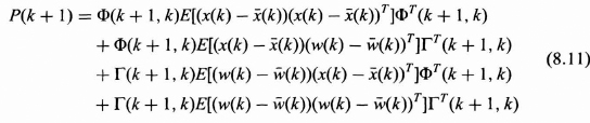
To finish the proof, we must show that the middle two terms of (8.11) are zero.
First let us look at the correlation between x(k) − ![]() (k) and w(k) −
(k) and w(k) − ![]() (k). Substituting (8.3) and (8.5) for x(k) and
(k). Substituting (8.3) and (8.5) for x(k) and ![]() (k) into E[(x(k) −
(k) into E[(x(k) − ![]() (k))(w(k) −
(k))(w(k) − ![]() (k))T] gives
(k))T] gives
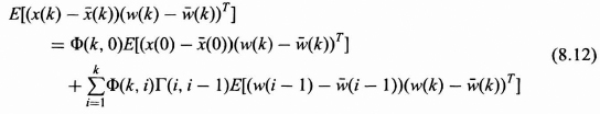
By the assumption (8.6), the first term on the right side of (8.12) is zero. Also since the summation of the second term goes only to k, the expected value of each term of the summation is zero by the assumption (8.7) and thus
![]()
This states that the x(k) − ![]() (k) and w(k) −
(k) and w(k) − ![]() (k) are orthogonal. Taking the transpose of (8.13), we also see that the third term of (8.11) is also zero and thus (8.9) is verified.
(k) are orthogonal. Taking the transpose of (8.13), we also see that the third term of (8.11) is also zero and thus (8.9) is verified.
8.2.2 Markov Sequence Model
In this section we define the Markov sequence model that is used in the development of the Kalman filter. The vector Markov sequence x(k) is defined as the output of a dynamic system to a vector white noise process w(k) as
![]()
In Eq. (8.14) the Φ[k + 1, k] is an n by n matrix, Γ[k + 1, k] is an n by p matrix, and w(k) is a p by 1 white vector sequence characterized by its covariance matrix Q(k) as follows:
Since w(k) is a p by 1 vector, the covariance matrix, Q(k), is a p by p positive definite matrix but is not necessarily diagonal at each k as we will allow correlation between components of the w(k) vector with this model. The fact that Q(k) is a function of k allows certain nonstationary processes to be included in the model.
The initial condition vector x(0) is assumed to be a random n vector characterized by its n by one mean vector, E[x(0)], and n by n covariance matrix, P(0), which are defined by
Furthermore we will assume that the white sequence w(k) is uncorrelated for all k with the initial condition vector x(0), that is,
![]()
This assumption is reasonable for most situations and will simplify considerably the work and the results that follow.
8.2.3 Observation Model
The state of the system (usually a random vector) is not directly available to us but is usually observed through a linear operation and contaminated with additive noise. So a reasonable model for the observation or measurement is
![]()
where
z(k + 1) is an m vector specifying the observation (measurement) vector at time k + 1.
x(k + 1) is an n vector representing the state vector of the system at time k + 1.
H(k + 1) is an m × n matrix called the measurement matrix at time k + 1.
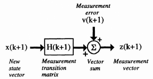
Figure 8.3 Vector block diagram for the observation model.
v(k + 1) is an m vector representing the measurement error at time k + 1.
x(0) is the initial condition with mean ![]() (0) and covariance matrix P(0).
(0) and covariance matrix P(0).
A vector block diagram for the observation process is shown in Figure 8.3. The observation error vector v(k + 1) is assumed to be a white random process with mean and covariance matrix defined by
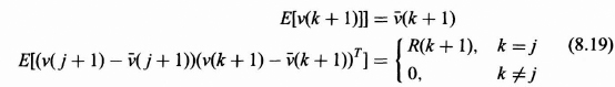
The R(k) is an m by m covariance matrix that is not necessarily diagonal and could be a function of the time index k. Thus v(k), the measurement error vector, is not necessarily required to be a stationary process.
Assume further, and quite reasonably so, that v(k + 1) is uncorrelated with the state initial condition, x(0), which can be expressed by
![]()
and that v(k + 1) is uncorrelated with w(j + 1) for all j and k as follows:
![]()
8.3 BASIC ESTIMATION PROBLEM
It is assumed that the state of the system that we desire to estimate is modeled as a Gaussian Markov sequence given by the following matrix difference equation from Eq. (8.14) with properties given in Section 8.2.2:
![]()
In most cases the states of the system themselves may not be directly measurable without error. We will assume that we have available z(k + 1), where z(k + 1) is given by
![]()
whose properties of v(k + 1) are given in Section 8.2.3. The z(k + 1) is called the observation or measurement vector, which is assumed to be an m vector, H(k + 1) is an m by n matrix relating the observation vector to the state vector, and v(k + 1) is an m vector representing the observation or measurement error.
8.3.1 Problem Formulation
The basic problem of estimation can now be formulated. Given the observation vectors at times 1, 2, …, j as z(1), z(2), …, z(j), determine an estimate of the state vector x(k) as a function of those observations. Let ![]() (k|j) represent the estimate of x(k) given z(1), z(2), …, z(j), that is,
(k|j) represent the estimate of x(k) given z(1), z(2), …, z(j), that is,
![]()
Depending on the relative positions of the time indexes k and j, we can identify three major types of estimation problems:
If k > j, the problem is prediction.
If k = j, the problem is filtering.
If k < j, the problem is smoothing or interpolation.
In making the estimate of x(k) given j observation vectors, an error is usually made. Define this estimation error vector ε(k|j) as follows:
![]()
Because x(k) and ![]() (k|j), which is a function of z(j), are random vectors, this error being the difference is also a random vector. A convenient measure of performance for the estimates is the expected value of some function C of the error:
(k|j), which is a function of z(j), are random vectors, this error being the difference is also a random vector. A convenient measure of performance for the estimates is the expected value of some function C of the error:
![]()
We desire then to find a function g(.), shown in Eq. (8.24), of the measurements z(0), z(1), …, z(j) such that J is minimized. Such an estimate is called the best or optimal estimate with respect to J. Different selections of C(.) may result in different estimates. For the purpose of this chapter, C(ε(k|j)) will be assumed to be C(ε(k|j)) = εT(k|j))ε(k|j), which gives rise to the minimum mean squared error estimates.
The choice of the g(.) can also result in different types of estimators including linear, nonlinear, time-invariant, and time-varying solutions. We will concentrate on linear time-varying estimates as discussed in the following section.
8.3.2 Linear Estimation with Minimum Mean Squared Error Criterion
In many cases a linear estimate is desired. It will be shown, first, that it is easy to implement, second, that theoretical results can usually be obtained for the performance before the procedure is implemented, and third, that only the first- and second-order properties of the measurement errors and state vector are needed to determine the estimator.
Assume that the g(.) is a linear function of the measurement vectors given in Eq. (8.23) represented by a matrix multiplication of the observations z(1), z(2), …, z(j). For convenience let z*(j) be the j · m column vector of measurements composed of the stacked observation vectors z(k) at times k = 1, 2, …, j given by
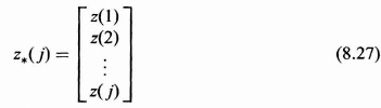
Since each z(k) is an m vector, z*(j) will be a j · m column vector, and its size will increase as j is increased. We can therefore write our estimate ![]() (k|j) as
(k|j) as
![]()
Where A is an n by j · m matrix called the coefficient matrix and b is an n by 1 constant vector. Assume for convenience that x(k) and v(k) are zero mean. If this is not the case, we may subtract off the mean vectors from the observation vectors and work with the new measurements without loss in generality. For the mean squared error performance criterion, assume that C(x) in (8.26) is expressed by C(x) = xT x. Thus J becomes
![]()
By this assumption, b can be shown to be a zero vector, and the problem reduces to finding a matrix A such that J is minimized. Since x(k) and z(k) are zero-mean stochastic sequences, the orthogonality principle can be applied to yield
![]()
where the zero matrix on the right side is an n by m · k zero matrix with elements all zero. Also from the orthogonality principle the minimum mean squared error is given by
![]()
Substituting (8.28) into (8.30) with b = 0, we have
![]()
Taking the expected value of the bracketed term and rearranging gives
![]()
Finally, solving Eq. (8.33) for the coefficient matrix A yields
![]()
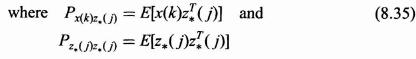
The optimal linear estimate ![]() (k|j) in the minimum mean squared error sense can thus be written as
(k|j) in the minimum mean squared error sense can thus be written as
![]()
To get the estimate, we must invert ![]() which is a jm by jm matrix. As j the number of observation vectors increases, this matrix size increases and for most large j becomes impractical to invert. What is desired from an engineering point of view are efficient and practical algorithms for evaluating optimum estimates
which is a jm by jm matrix. As j the number of observation vectors increases, this matrix size increases and for most large j becomes impractical to invert. What is desired from an engineering point of view are efficient and practical algorithms for evaluating optimum estimates ![]() (k|j). We will see later in this chapter that if certain assumptions are placed on properties of the measurement error vector v(k + 1) and the message model source u(k) that sequential algorithms, the Kalman filter [14], exist for practical implementation of the estimates. It has been shown by Meditch [1] that the estimate forms are optimal for other forms of L and that the linear estimates are also optimum nonlinear filters if the processes are all Gaussian.
(k|j). We will see later in this chapter that if certain assumptions are placed on properties of the measurement error vector v(k + 1) and the message model source u(k) that sequential algorithms, the Kalman filter [14], exist for practical implementation of the estimates. It has been shown by Meditch [1] that the estimate forms are optimal for other forms of L and that the linear estimates are also optimum nonlinear filters if the processes are all Gaussian.
8.4 OPTIMAL FILTERED ESTIMATE
One of the most basic problems in communication theory is the filtering of a noisy signal to obtain a cleaner version of the signal. In general, the signal could represent a voltage, current, position, velocity, acceleration, or any combination. In Chapter 7 the optimal linear filter under the Wiener framework was found. Procedures were described for the estimation of a single scalar signal, assuming that the signal and noise are modeled as wide sense stationary processes characterized by their autocorrelation functions and power spectral densities. The extension to the nonstationary case and vector processes was not accomplished because of a complexity that borders on impossibility. The Kalman filter can easily handle nonstationary and vector processes because of its basic state space formulation. The signals and nonstationarities must be, however, within the signal model and linear state space formulation, and the noise process must be of the additive form and in particular assumed to be white.
8.4.1 The Kalman Filter
In the Kalman formulation we desire the best linear estimate of the state vector x(k) as a function of the observation vectors z(1), z(2), …, z(k), where best is assumed to be in the minimum mean squared error sense. It can be shown that the Kalman filter is optimum under a wider class of performance functions than the mmse function.
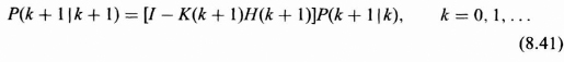
Let ![]() (k|k) represent the estimate of the state at time index k given observations z(1), z(2), …, z(k). The Kalman filter thus gives us a running estimate of the state at time index k as a function of the observations as shown conceptually in Figure 8.4.
(k|k) represent the estimate of the state at time index k given observations z(1), z(2), …, z(k). The Kalman filter thus gives us a running estimate of the state at time index k as a function of the observations as shown conceptually in Figure 8.4.
The Kalman filter and associated sequential algorithms for prediction and smoothing will be presented, theorem like, specifying clearly the given assumptions, the form of the optimal filter, and the performance associated with the optimum filter. Proofs will not be given. The overall presentation of results summarizes those given in Meditch [1]. Students interested in seeing the proofs can find them in many references, in particular, Meditch [1] and Kalman and Bucy [13].
KALMAN FILTER SUMMARY
Assumptions
The state of the system is governed by the model in Section 8.2.2. It is assumed that Φ(k + 1, k), Γ(k + 1, k), P(0), and Q(k) are known and deterministic. It is assumed that the observation model is given in Section 8.2.3 with H(k + 1) and R(k) known and deterministic. These are summarized as follows:

Kalman Filter Algorithm: Filtered Estimate
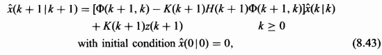
The optimal linear filtered estimate ![]() (k + 1|k + 1) as shown by Kalman [13] to be governed by the recursive matrix formula for
(k + 1|k + 1) as shown by Kalman [13] to be governed by the recursive matrix formula for

where K(k + 1) is called the Kalman gain.
Kalman Gain
The Kalman gain is given by
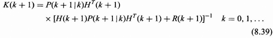
Notice that the Kalman gain is written in terms of a P(k + 1|k), which is the single-step prediction error covariance matrix, which is now defined.
Single-Step Prediction Error Covariance Matrix (Single-Step Performance)
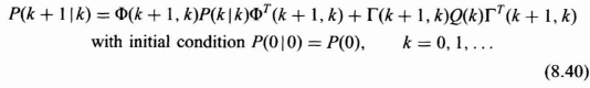
Error Covariance Matrix for Filtered Error (Covariance Recursion)
Performance (Covariance Matrix for Kalman Filtered Estimate of the State)

The diagonal components of P(k + 1|k + 1), the error covariance matrix, are the variances of the estimates of each individual component of the state vector x(k + 1), thus providing a measure of performance of the component estimates determined by the Kalman filter. This measure of effectiveness is available from Eq. (8.41) and can be calculated before any measurements are taken or processed. The off-diagonal components give the covariances of the error vector components. The state vector block diagram for the Kalman filtered estimate given in Eq. (8.38) is shown in Figure 8.5.
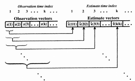
Figure 8.4 Timing diagram for the discrete Kalman Filter.
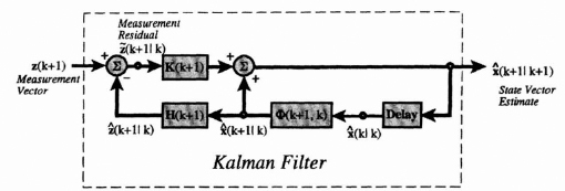
Figure 8.5 Vector block diagram for the Kalman Filter in terms of the measurement residual.
An alternative form of the Kalman filter can be derived from (8.38) by grouping together the ![]() (k|k) terms to get
(k|k) terms to get
This implementation of the Kalman filter is shown in Figure 8.6 as a first-order vector difference equation with the measurement vector as the driving function.
In the following sections the structure and the internal workings of the Kalman filter are explored.
8.4.2 The Anatomy of the Kalman Filter
From Eq. (8.38) we saw that the filtered estimate at time k + 1 in terms of k + 1 measurements is a function of the optimum estimate at time k using k measurements and the new measurement at time k + 1 as shown in Figure 8.7. The measurement residual ![]() (k + 1|k) is defined by the error in the predicted measurement as follows:
(k + 1|k) is defined by the error in the predicted measurement as follows:
![]()
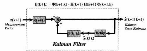
Figure 8.6 Alternative vector form of the Kalman Filter.
In Figure 8.7 sections of the filter equation are identified that illustrate how the Kalman filter works as a predictor-corrector. The filter first predicts the new state (single-step prediction) and then corrects it by adding the product of the Kalman gain and the measurement residual. The measurement residual is seen as the difference between the new measurement and the single-step prediction of the measurement. If they are the same then the residual will be zero and no correction is applied.
8.4.3 Physiology of the Kalman Filter
From Eq. (8.38) it is seen that the new estimate is a function of the state transition matrix, Φ(k + 1|k), the measurement matrix, H(k + 1), the old estimate ![]() (k|k), the new measurement z(k + 1), and the Kalman gain K(k + 1). Of these only the Kalman gain needs to be calculated. The Kalman gain matrix (possibly different at each time index) is determined by the coupled Eqs. (8.39) to (8.41), which specify a recursive evaluation of P(k + 1|k), K(k + 1), and P(k + 1|k + 1). This recursion displayed in Figure 8.8 shows that the P(k + 1|k), K(k + 1), and P(k + 1|k + 1) must be calculated in that order.
(k|k), the new measurement z(k + 1), and the Kalman gain K(k + 1). Of these only the Kalman gain needs to be calculated. The Kalman gain matrix (possibly different at each time index) is determined by the coupled Eqs. (8.39) to (8.41), which specify a recursive evaluation of P(k + 1|k), K(k + 1), and P(k + 1|k + 1). This recursion displayed in Figure 8.8 shows that the P(k + 1|k), K(k + 1), and P(k + 1|k + 1) must be calculated in that order.
In Eq. (8.39) to (8.41) notice that P(k + 1|k), K(k + 1), and P(k + 1|k + 1) do not depend on the measurements or estimates. Thus they can be calculated “off line” before they are needed, or in “real time” as the measurements come in. If they are calculated ahead of time there is no overhead for their calculation, but storage must be provided for all the K(k + 1) determined for all k that the filter is to be used. If we calculate them between the presentation of observations, the acceptable sample rate may have to be reduced because of the extra computational load.
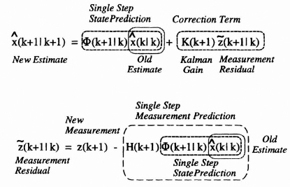
Figure 8.7 Predictor-corrector structure of the Kalman filtering equation.
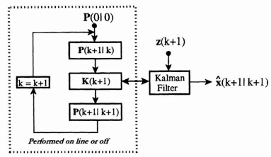
Figure 8.8 Recursive calculation procedure for the prediction error covariance, the Kalman gain, and the filtered error covariance matrices.
It is also interesting to note that the performance characteristics given by P(k + 1|k + 1), the error covariance matrix for estimating the state, can be determined without a single measurement. Thus the overall performance of the Kalman filter can be easily computed before any implementation.
A simple one-dimensional or scalar filtering problem is now presented.
EXAMPLE 8.1
The message and observation models are given as follows
![]()
Assume that R and Q are given by
![]()
Find the Kalman filter for estimating the signal x(k + 1) from the given k + 1 measurements.
SOLUTION
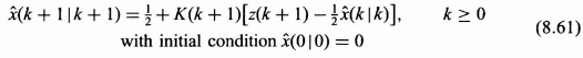
Since the state vector is just one dimensional, the Kalman filter in the scalar form of Eq. (8.38) can be written as follows, with initial condition ![]() (0|0) = 0:
(0|0) = 0:
![]()
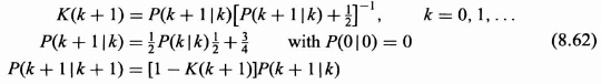
where the K(k + 1), P(k + 1|k), and P(k + 1|k + 1) are determined from (8.39) to (8.41) for k = 0, 1, 2, … as
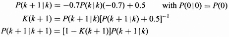
For the order shown above and P(0|0) = 10, the values for the P(k + 1|k), K(k + 1), and P(k + 1|k + 1) are calculated. The graph of each is plotted in Figure 8.9.
Notice that the Kalman gain is dynamic for the first few terms but quickly reaches a steady state result of 0.5603575. The P(k + 1|k) approaches a steady state value of 0.6372876. This gives the single-step prediction error. The P(k + 1|k + 1) starts out high and approaches quickly a steady state value of 0.2801788 which represents the mean squared error for the filtered estimate in the steady state.
Also note that the form of the Kalman filter is determined without the knowledge of the measurements and thus can be computed offline if desired before any measurements are taken. ![]()
EXAMPLE 8.2
In this example we begin with an AR(2) model for a signal x(k), which is given by
![]()
with E[w(k)w(j)] = δ(j − k). We observe x(k) in additive white noise v(k), with an autocorrelation function RVV(k − j) = δ(j − k). We want to estimate the scalar signal x(k) using a Kalman filter. Find the message and observation models for this estimation problem, and specify the Kalman filter that performs the desired estimation of x(k).
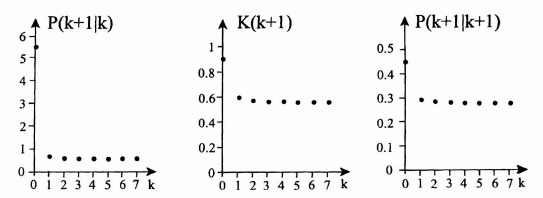
Figure 8.9 Plots of P(k + 1|k), K(k + 1), and P(k + 1|k + 1) for Example 8.1.
SOLUTION
Although the signal we wish to estimate is a scalar, the state variable formulation results in a vector formulation because of the delay of two samples in the model. To obtain the state variable representation, let the first state variable be x1(k) = x(k), what we wish to estimate, and the second be x2(k) = x(k − 1). This choice of state variables facilitates the development of the state model. Any other assignment can be made giving a different filter form, yet the resulting filter will give equivalent performance. Since the Kalman filter estimates the state of the system, we will simultaneously estimate both x(k) and x(k − 1). Evaluating the AR(2) model given above at k + 1 gives
![]()
By the definitions for x1(k) and x2(k), this equation can be rewritten as
![]()
The second equation for the state model is obtained from the definitions of x1(k) and x2(k) as
![]()
These two equations can be put in the standard state variable form, resulting in the following message model:
![]()
Since v(k + 1) is the additive noise and we observe only z(k + 1) = x(k + 1) + v(k + 1), the measurement model can be written as
![]()
The model is now in the standard form for application of the Kalman filter. The model parameters are
![]()
The Q associated with the message model w(k) and the R associated with the additive measurement noise model v(k) are, respectively, Q = 1 and R = 1 from the given autocorrelation functions of w(k) and v(n). To complete the model, initial conditions on the state at the origin and the state covariance at the origin must be assigned. These initial values are assigned as follows:
![]()
P(0|0) is arbitrarily selected, usually with large values on the main diagonal, whereas the zero vector for x(0) comes from the fact that the signal has a zero mean, since it is generated from a white source which implies a zero mean.
From the assumptions above and the definitions in Eqs. (8.39), (8.40), and (8.41), the P(k + 1|k), K(k + 1), and P(k + 1|k + 1) for the Kalman filter are determined as follows:
The Kalman filter in terms of P(k + 1|k), K(k + 1), and P(k + 1|k + 1) and the model parameters from (8.38) becomes
By collecting the terms for ![]() 1(k) and
1(k) and ![]() 2(k) and simplifying the equation above we can show the Kalman filter to be
2(k) and simplifying the equation above we can show the Kalman filter to be
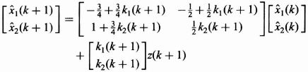
In this form the new vector estimate is written as a linear function of the previous estimates plus a linear function of the new measurement. Thus the Kalman filter recursively calculates both the estimate of x(k + 1), which is ![]() 1(k + 1) and x(k) which is
1(k + 1) and x(k) which is ![]() 2(k + 1) given the k + 1 measurements.
2(k + 1) given the k + 1 measurements. ![]()
The procedure described in establishing the state model that of using delayed versions of the message signal as states can be used for an AR model of any order. An AR(p) model leads to a p by p state transition matrix. The state assignments for an ARMA(p, q) model can be done in many different ways, all of which lead to alternative, but equivalent, forms for estimating the ARMA signal in additive noise.
8.5 OPTIMAL PREDICTION
Prediction is the process of estimating a process in future time from current and past measurements. There are many practical problems that require prediction. For example, we may have data representing measurements of position, velocity, and acceleration of an object in space and desire to “predict” where the object will be at a certain time into the future, and also what its velocity and acceleration are at that time. Another example is that we may have measurements of a random processes and wish to estimate the value of the process at times advanced from the present like a stock market projection. There are two main basic types of predictors based on where in the future the predictions occur; they are (a) fixed lead prediction and (b) fixed point prediction.
8.5.1 Fixed Lead Prediction
Suppose that we have available measurements z(1), z(2), …, z(k) that are somehow statistically related to the state vector, x(k), for all k, and that we desire the fixed lead prediction or estimation of the state vector x(k + N) given by ![]() (k + N|k). The N, which is a fixed integer, represents the lead time for the prediction. In fixed lead prediction, each time we accept a new measurement, we are always predicting a fixed amount ahead in time using all the measurements. This is illustrated in Figure 8.10. From the figure we see that at time index k, we observe z(1), z(2), …, z(k) to estimate x(k + N). Similarly, at time index k + 1, we use all the previous measurements z(1), z(2), …, z(k) and the new measurement z(k + 1) to estimate x(k + 1 + N). This process is continued for all time indexes.
(k + N|k). The N, which is a fixed integer, represents the lead time for the prediction. In fixed lead prediction, each time we accept a new measurement, we are always predicting a fixed amount ahead in time using all the measurements. This is illustrated in Figure 8.10. From the figure we see that at time index k, we observe z(1), z(2), …, z(k) to estimate x(k + N). Similarly, at time index k + 1, we use all the previous measurements z(1), z(2), …, z(k) and the new measurement z(k + 1) to estimate x(k + 1 + N). This process is continued for all time indexes.
If we restrict the form of the predictor to be linear, as in the linear state model, and assume that our observations are the sum of linearly transformed states and a white noise process, then the optimal fixed lead predictor can be shown to be expressed in the following summary. The presentation is composed of three main parts: basic assumptions, the optimal algorithm, and the performance of the optimal predictor measured by the mean squared error.
OPTIMAL FIXED LEAD PREDICTOR SUMMARY
Assumptions
Let the state of the system be governed by the Markov sequence model given in section 8.2.2 with known deterministic Φ(k + 1, k), Γ(k + 1, k), P(0), and Q(k), and let the observation model be as given in Section 8.2.3 with known deterministic H(k + 1) and R(k). These assumptions are summarized as follows:
Fixed Lead Prediction Algorithm
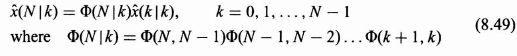
The optimal fixed lead predictor ![]() (k + N|k) with lead time N can be shown to be
(k + N|k) with lead time N can be shown to be
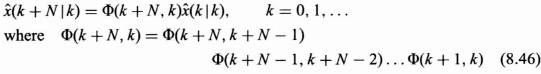
and ![]() (k|k) is the optimal linear filtered estimate of the state at time index k obtained from the Kalman filter (Eq. 8.38) using initial conditions
(k|k) is the optimal linear filtered estimate of the state at time index k obtained from the Kalman filter (Eq. 8.38) using initial conditions ![]() (0|0) and P(0|0) = P(0).
(0|0) and P(0|0) = P(0).
Performance
The performance specified by the error covariance matrix can be shown from Meditch [1] to be
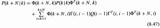
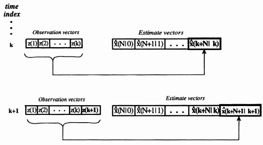
Figure 8.10 Fixed lead prediction using all data in the past.
Recursive formulas can be derived for the determination of the sum term as well as for the generation of the Φ(k + N, k) term from previous terms if desired, but as this can be determined off line, it is not necessary unless implementing directly on line.
8.5.2 Fixed Lead Prediction (Sliding Window)
Because of memory limitations there are cases where only a certain portion of the past measurements are used to perform the estimation. The most common of this type is the sliding window fixed lead prediction which uses only the previous W indexed measurements, where W is the length of the sliding window. Such algorithms will not be presented in our discussion, and Van Trees [16] can be consulted for a thorough discussion of sliding window estimators.
8.5.3 Fixed Point Prediction
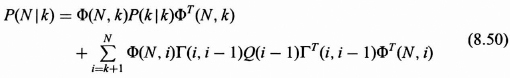
In fixed point prediction a time index is selected or fixed, say at N, and estimates of the state at time N are made using successive observations up to that time. This process generates a running estimate of the state at time N, ![]() (N|k) for k = 0, 1, 2, …, N − 1, as illustrated in Figure 8.11.
(N|k) for k = 0, 1, 2, …, N − 1, as illustrated in Figure 8.11.
At time index 1 we observe z(1) and predict x(N) with ![]() (N|1), and next for time index 2 we use both observations z(1) and z(2) to predict x(N) with
(N|1), and next for time index 2 we use both observations z(1) and z(2) to predict x(N) with ![]() (N|2) This process is continued until we observe z(1), z(2), …, Z(N − 1) to predict x(N) with
(N|2) This process is continued until we observe z(1), z(2), …, Z(N − 1) to predict x(N) with ![]() (N|N − 1). If further observations are included, the problem is no longer that of prediction but that of filtering for k = N and smoothing for k > N.
(N|N − 1). If further observations are included, the problem is no longer that of prediction but that of filtering for k = N and smoothing for k > N.
The summation term can be obtained recursively by subtracting the relevant term in the summation each time from the previous sum if desired.
OPTIMUM FIXED POINT PREDICTOR SUMMARY
Assumptions: Same as for Fixed Lead Predictor
The state of the system is governed by the model given in Section 8.2.2 with known deterministic Φ(k + 1, k), Γ(k + 1, k), P(0), and Q(k), and the observation model is as given in Section 8.2.3 with known deterministic H(k + 1) and R(k). These are summarized as follows:

Fixed Point Predictor Algorithm
The optimal fixed point predictor for estimating x(N), given measurements up to time k is defined by ![]() (N|k), where N is a fixed constant. The algorithm for obtaining
(N|k), where N is a fixed constant. The algorithm for obtaining ![]() (N|k) follows:
(N|k) follows:
The ![]() (k|k) in the predictor algorithm is the optimal linear filtered estimate of the state at time index k obtained from the Kalman filter (Eq. 8.38) with
(k|k) in the predictor algorithm is the optimal linear filtered estimate of the state at time index k obtained from the Kalman filter (Eq. 8.38) with ![]() (0|0) = 0 and P(0|0) = P(0).
(0|0) = 0 and P(0|0) = P(0).
Performance: Error Covariance Matrix
8.6 OPTIMAL SMOOTHING
Smoothing is the term used to describe estimation of the state of the system at time index k using measurements from the beginning at 1 up to the time index j where j is greater than k. The estimator uses measurements both before and after k and thus is inherently a noncausal form of processing. Because of this extra flexibility, there are several forms of smoothing algorithms including: fixed interval, fixed point, and fixed lag smoothing.
In fixed interval smoothing the purpose is to determine the estimate of the state at all time indexes k = 0, 1, 2, …, N − 1 for a fixed interval length of N. This is a nonreal time form of processing.
For fixed point smoothing we desire the estimate of the state at some time index N using all measurements up to time index N + 1, then up to N + 2 and so on. In this way we obtain running estimates of the state at time N as we accept more and more measurements. Although noncausal in the sense of providing estimates at times in terms of future measurements, the algorithm can be developed to operate in pseudo real time in a recursive fashion as the measurements come in.
Figure 8.11 Fixed point prediction timing diagram.
Fixed lag smoothing gives the smoothed estimate at successive time indexes k in terms of all measurements up to k + L, where L represents the time lag behind the measurements. Fixed lag smoothing can also be obtained in a recursive fashion and in real time if we accept a time lag.
Each of these forms of smoothing is explored in the following sections as the details of the optimal smoothing algorithms are presented.
8.6.1 Fixed Interval Smoothing
In fixed interval smoothing we desire the estimates of the state of the system for all values of time index, k = 0, 1, …, N − 1, where N is the length of the fixed time interval over which data are processed. Conceptually this is shown in Figure 8.12.
The optimal linear fixed interval smoothing estimators, where optimality is in the sense of minimizing the mean squared error, can be obtained by a development similar to that used for obtaining the filtered estimate in Section 8.4.1. However this procedure requires the calculation of a different coefficient matrix for each k in evaluating ![]() (k|N) and correspondingly the evaluation of inverses of large matrices for large N. It does not take a very large N to make this particular approach not only computationally intensive but virtually impossible.
(k|N) and correspondingly the evaluation of inverses of large matrices for large N. It does not take a very large N to make this particular approach not only computationally intensive but virtually impossible.
In the literature, recursive algorithms for calculating the smoothed estimates have been developed because of the unique framework induced by the state and measurement models. Most of the algorithms are seen to include the determination of the Kalman filtered estimates in a forward recursive formulation and the determination of the smoothed estimates in a backward recursive formulation. The following presentation is given without proof and summarizes the algorithm given by Meditch [1].
OPTIMAL FIXED INTERVAL SMOOTHING SUMMARY
Assumptions
The state of the system is governed by the model given in Section 8.2.2 with known deterministic Φ(k + 1, k), Γ(k + 1, k), P(0), and Q(k), and the observation model is as given in Section 8.2.3 with known deterministic H(k + 1) and R(k). These are summarized as follows:

Algorithm (Fixed Interval Smoothing)
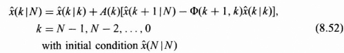
The smoothing gain, A(k), is determined as follows:
![]()
where P(k|k) and P(k + 1|k) are the same as those determined from the Kalman filter. Thus A(k) can be calculated by using the recursive calculation of P(k|k) and P(k + 1|k) as shown in Figure 8.8 and described by Eqs. (8.39) to (8.41).
Performance
The error covariance matrix P(k|N) defined by
![]()
is determined by a backward recursion as follows:

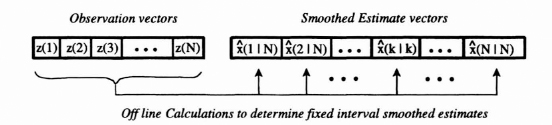
Figure 8.12 Conceptual diagram for fixed interval smoothing.
The P(N|N) is obtained in the forward calculation from the Kalman filter. From examination of the algorithm’s equations (8.52 and 8.55), we see that it uses measurements in a forward recursion to obtain the filtered estimate for all k indexes in the entire fixed interval N, and then uses these Kalman filtered estimates in a backward recursion to generate the smoothed estimates at time indices N − 1, N − 2, and so on. This procedure is shown conceptually in Figure 8.13. In the figure the KF represents the Kalman filtering operation described in Eqs. (8.38) to (8.41), and the SM represents the smoothing algorithm just described in Eq. (8.52). Note that the initial condition for the forward direction is ![]() (0|0), which is a zero vector, and that the initial condition in the backward direction is
(0|0), which is a zero vector, and that the initial condition in the backward direction is ![]() (N|N), the filtered estimate at time index N, which uses all the data up to and including time index N.
(N|N), the filtered estimate at time index N, which uses all the data up to and including time index N.
The performance of the optimum smoothed estimates is given in Eq. (8.55) as it gives the error covariance matrix for the estimates ![]() (k|N). This performance can be calculated “off line” as it is not a function of the measurements as was the case for the Kalman filter performance. By virtue of having additional measurements in the calculation of the estimates, the entries on the diagonals of P(k|N) are less than the corresponding entries in P(k|k). The difference of the corresponding elements on the diagonals, P(k|N) − P(k|k), represents the gain in performance for estimating the components of the state vector x(k) by using the smoothing algorithm rather than the filtered algorithm.
(k|N). This performance can be calculated “off line” as it is not a function of the measurements as was the case for the Kalman filter performance. By virtue of having additional measurements in the calculation of the estimates, the entries on the diagonals of P(k|N) are less than the corresponding entries in P(k|k). The difference of the corresponding elements on the diagonals, P(k|N) − P(k|k), represents the gain in performance for estimating the components of the state vector x(k) by using the smoothing algorithm rather than the filtered algorithm.
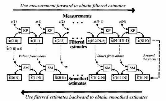
Figure 8.13 Conceptual calculation procedure for the Fixed Interval Smoothed estimates indicating forward and backward recursion.
8.6.2 Fixed Point Smoothing
Fixed point smoothing is the process of estimating the state of the system at some fixed time index K as the observation index j increases from K + 1. This overall operation is indicated in Figure 8.14.
In this figure the first line indicates that z(1), z(2), …, z(K + 1) are used to estimate x(K) by ![]() (K|K + 1), the second line indicates that z(1), z(2), …, z(K + 1) are used to estimate x(K) by
(K|K + 1), the second line indicates that z(1), z(2), …, z(K + 1) are used to estimate x(K) by ![]() (K|K + 2), and so on. This process is continued as long as there are new inputs.
(K|K + 2), and so on. This process is continued as long as there are new inputs.
One way of implementing fixed point smoothing is by performing successively the Kalman filter to obtain ![]() (K + 1|K + 1), and then the fixed interval smoothing algorithm of size K + 1 to obtain
(K + 1|K + 1), and then the fixed interval smoothing algorithm of size K + 1 to obtain ![]() (K|K + 1) by iterating one step back from the filtered estimate. Similarly, to get
(K|K + 1) by iterating one step back from the filtered estimate. Similarly, to get ![]() (K|K + 2), we perform successively the Kalman filter to obtain
(K|K + 2), we perform successively the Kalman filter to obtain ![]() (K + 2|K + 2), and then the fixed interval smoothing algorithm of size K + 2 to obtain
(K + 2|K + 2), and then the fixed interval smoothing algorithm of size K + 2 to obtain ![]() (K|K + 2) by iterating two steps back from the filtered estimate. As further measurements are taken in, it is necessary to iterate further and further back. A more efficient algorithm has been developed (see Meditch [1]), and it is now described without proof in the following fixed point presentation. This algorithm determines the required estimates recursively using the previous estimate at the fixed point and the two filtered estimates at the running indexes j and j − 1 as shown in Eq. (8.56).
(K|K + 2) by iterating two steps back from the filtered estimate. As further measurements are taken in, it is necessary to iterate further and further back. A more efficient algorithm has been developed (see Meditch [1]), and it is now described without proof in the following fixed point presentation. This algorithm determines the required estimates recursively using the previous estimate at the fixed point and the two filtered estimates at the running indexes j and j − 1 as shown in Eq. (8.56).
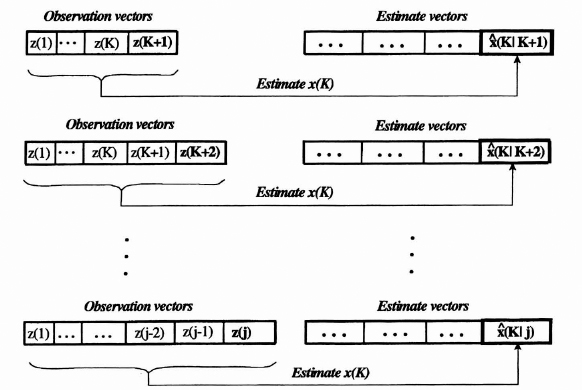
Figure 8.14 Timing diagram for the fixed point smoothing algorithm.
FIXED POINT SMOOTHING SUMMARY
Assumptions
The state of the system is governed by the model given in Section 8.2.2 with known deterministic Φ(k + 1, k), Γ(k + 1, k), P(0), and Q(k), and the observation model is as given in Section 8.2.3 with known deterministic H(k + 1) and R(k). These are summarized as follows:
Fixed Point Smoothing Algorithm
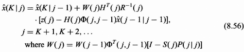
The initial condition is W(K) = P(K|K).
Performance
The error covariance matrix P(K|j) is defined by
![]()
It is determined from
![]()
8.6.3 Fixed Lag Smoothing
Fixed lag smoothing gives the estimate of the state of the system at time index k as a result of measurements taken up to the time index k + L, where L is a fixed lag and k runs from one to infinite. This process is illustrated in Figure 8.15.
It is possible to obtain the fixed smoothed lag filter by using the fixed interval smoothing algorithm for each new iteration and a step back to obtain the smoothed estimate at the desired lag. Recursive algorithms have been developed for the fixed lag smoothed estimate, and in general, they are quite complex. If desired consult Meditch [1] for details.
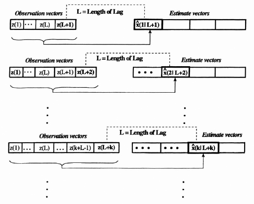
Figure 8.15 Timing diagram for the fixed lag smoothed estimates.
8.7 STEADY STATE EQUIVALENCE OF THE KALMAN AND WIENER FILTERS
In general, the Kalman filter is different from the Wiener filter, although both are optimum linear filters for estimating signals. A big difference is in the main formulation where the Kalman filter is described for time index n greater than or equal to zero, whereas the Weiner filter assumes that the processes are defined for all indexes of time. The resulting Kalman filter thus contains an initial transient as part of its solution, while the Weiner filter is assumed to be steady state. The standard Weiner filter works for estimating random processes that are wide sense stationary, while the Kalman filter inherently estimates nonstationary processes. The Kalman filter is described in a state variable form. Thus it is able to handle optimum estimation of vector processes, while the Wiener filter is very cumbersome mathematically, bordering on impossibility, for handling vector processes.
The following example will illustrate a form of equivalence of the Kalman steady state filter and the Weiner filters for estimating a signal process in noise with comparatively equal first-order scalar models, each described in a different framework.
8.7.1 Kalman Filter Formulation
Suppose that a scalar random process x(k) is observed in additive white noise and that the signal and observation are mathematically modeled as follows:
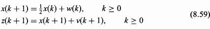
The following assumptions are made with respect to the characterization of the w(k), the signal generation white noise process, and v(k), the additive white noise process:
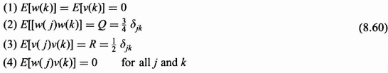
These assumptions are consistent with those for the Kalman filter. They are described in terms of expected values of various time domain products. We wish to find the optimal estimate ![]() (k + 1) of the signal process by a linear filter where optimality is in the minimum mean squared error sense.
(k + 1) of the signal process by a linear filter where optimality is in the minimum mean squared error sense.
From (8.59) and (8.60) the given values of the message and observation models are seen to be not a function of k and determined as Φ = ![]() , Γ = 1, H = 1, R =
, Γ = 1, H = 1, R = ![]() , and Q =
, and Q = ![]() . Substituting these parameters into Eq. (8.38) gives the Kalman filter as
. Substituting these parameters into Eq. (8.38) gives the Kalman filter as
where K(k + 1), P(k + 1|k), and P(k + 1|k + 1) are given from (8.39 to 8.41) by
Remember that the order of computation is P(k|k) → P(k + 1|k) → K(k + 1) → P(k + 1|k + 1) starting with k = 0 and continuing with k = 1, 2, …. If it is assumed that a steady state has been reached, then the K(k + 1), P(k + 1|k), and P(k|k) all will be constants and defined as follows:
![]()
Substituting the steady state filter parameters from (8.63) into (8.62) gives the following:
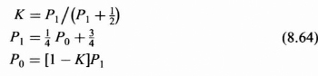
Equation (8.64) gives us three nonlinear equations in terms of K, P1, and P0. They can be solved to give
![]()
Using the steady state filter values of (8.65) in (8.61), gives the steady state Kalman filter as follows:
![]()
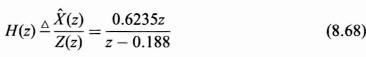
The transfer function H(z) for the Kalman filter can be determined by taking the Z-transform of (8.66) to yield
![]()
Solving for ![]() (z) over Z(z), which is the transfer function H(z) for the steady state Kalman filter for this problem, we obtain
(z) over Z(z), which is the transfer function H(z) for the steady state Kalman filter for this problem, we obtain
We now pose the problem so that a Wiener filter can be obtained and find the optimal filter using the Wiener formulation.
8.7.2 Wiener Filter Formulation
The Wiener filter is an optimum linear time-invariant filter for estimating one signal process x(n) from an observed process z(n), where optimality is in the minimum mean squared error sense. The information required to obtain the optimal filter is in terms of the autocorrelations and cross correlations of the processes involved, or equivalently in the frequency domain in terms of the auto- and cross-spectral densities of the processes. It is assumed that the observed process z(k) is the sum of the signal process x(k) and a white noise process v(k) as
![]()
The difference between this part of the Wiener formulation and the Kalman filter formulation (8.59) is that (8.69) is assumed to hold for all time rather than just at times greater than or equal zero. To make the models otherwise equal, we need to select the properties of v(k) and x(k) to be equivalent to the Kalman formulation, that is,
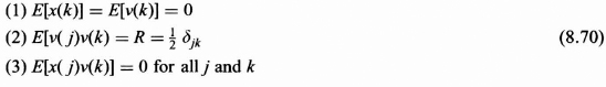
The third assumption is that the signal process x(j) is uncorrelated with the noise process v(k), which is similar to the uncorrelated property of the w(k) in the Kalman formulation. It is also required that the signal process x(k) be somehow equivalent to the state variable representation given in the Kalman formulation. In general, the Kalman filter has a time-varying autocorrelation function as a result of the governing state model starting at zero. So, for equivalence of this example, it is necessary to assign the steady state autocorrelation function to the signal model for the Wiener formulation. The steady state autocorrelation function for the state model can be shown to be RXX(k) = (![]() )|k|, so the last assumption for the Wiener formulation is
)|k|, so the last assumption for the Wiener formulation is
![]()
Thus we specify the autocorrelation function or equivalently the power spectral density of the random process x(k) rather than the state model for its generation from white noise.
We would like to find the discrete time Wiener filter for estimating the x(k). From Chapter 7 (Eq. 7.101), the optimal discrete-time filter for estimating the desired G[n] = x(n) from the observed Z(n), each with rational spectra, has a transfer function H(z) given by
![]()
where ΨXZ(z) = Zβ(RXZ(k)) and ΨXX(z) = Zβ(RXX(k)), which are determined as


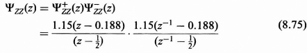
The ΨXZ(z) is then spectrally factorized as follows:
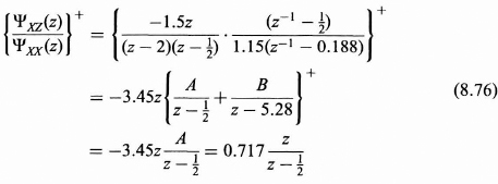
The next step is to obtain the + time part of the partial fraction expansion:
Finally, substituting (8.76) into (8.72), we find the transfer function H(z) for the optimum linear causal time-invariant filter to be
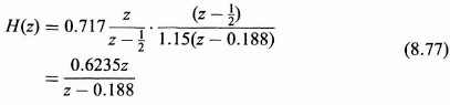
Thus the H(z) determined using the Kalman filter steady state formulation (8.68) and the H(z) determined using the Wiener filter formulation (8.77) are the same, which establishes the equivalence for this simple example. This type of steady state equivalence for wide sense stationary processes can also be established in general, but the proof is beyond the scope of our development for this chapter.
8.8 SUMMARY
In this chapter optimal discrete time linear systems were presented where optimality was with respect to the minimum mean squared error criterion. The optimal filters were written in terms of the parameters of the state variable representation of the message generation model and the parameters of an additive white noise observation model. The main result, the Kalman filter, was originally presented by R. E. Kalman [13, 14].
Our presentation begins with the establishment of the basic structure of the message and observation models. The message model was described in a state variable representation as the output of a linear, possibly time-varying, system to a white noise source input. This was the Markov sequence model. The observation model was assumed as a sum of a weighted white noise process and a linear combination of the states.
For these message and observation models the important problems of prediction, fitering, and smoothing were explored, and the procedures and formulas were presented for the optimum filters and their mean squared error performances.
The Kalman filter was presented without proof, and several examples were given to describe the process of obtaining the Kalman gain which, along with the filter form, determined the optimal filter. The filter form was expressed is in terms of the original message state model properties and was shown to be in a prediction-correction form. The first example presented was a one-dimensional filtering problem, while the second was the estimation of an AR(2) random process in additive noise. The state vector formulations for these examples were obtained by a reasonable assignment of the state variables, and this indicates the generality of the vector Markov message model.
Although our presentation did not include proofs, various different proofs for the Kalman filter exist in the literature. The interested reader should consult Kalman [14], Meditch [1], and Sage and Melsa [5] for their detailed versions.
The basic optimal filter structures, procedures, and performances for fixed interval fixed point, and fixed lag smoothing were presented without proof in a format similar to that given by Meditch [1]. Also presented, without proof, were optimal filters for obtaining the fixed point and fixed lead prediction estimates.
The chapter concludes with an example that illustrates a form of equivalence of the steady state Kalman filter and the Wiener filter. Since the Kalman filter is a time domain presentation and the Wiener filter is frequency based, care was needed in formulating the equivalent problems.
The presentation in this chapter has been limited to the discrete time Kalman filter formulation. A parallel theory is available for the continuous time Kalman filter. For a discussion of the continuous time Kalman filter, the reader can benefit from presentations by Kalman [13], Brown [10], Sage and Melsa [5], and Van Trees [16]. In many cases it is convenient to implement the continuous Kalman filter in discrete time allowing computer implementation. This usually requires obtaining a discrete time model for the continuous message model. Various techniques for handling this type of modeling have been established by the modern-day control theory community, and a good starting point for this area can be found in Cadzow and Martens [12].
The Kalman filter has been shown to be a little more general in terms of problems it can solve. Extensions include those for different performance measures than the mean squared error and different statistical representations than Gaussian. These properties are nicely presented in the text by Meditch [1].
Also the Kalman filter has been extended to nonlinear state models, and the procedures and formulas for implementation are given by Sage and Melsa [5], Anderson and Moore [4], and Candy [9]. The resulting filter structure, called the extended Kalman filter, is no longer linear and also not necessarily the optimum nonlinear filter either. Optimum nonlinear filters are outside the scope of this book.
PROBLEMS
8.1 A system model is given as
![]()
with the following assumptions:
(1) Initial condition is known and given by x(0) = [0, 0]T.
(2) w(k) is a scalar zero mean white Gaussian sequence with a known autocorrelation function given by E[w(j)w(k)] = δjk.
We are given the measurement model as
![]()
with the following assumptions:
(3) v1(k + 1) and v2(k + 1) are independent zero mean white Gaussian sequences with the properties
![]()
(4) w(k) is uncorrected with both measurement noise processes v1(k + 1) and v2(k + 1) for all j and k.
![]()
We wish to find the formulas governing the Kalman filter for the case of estimating the state vector x(k + 1) = x1(k + 1), x2(k + 1)]T from the measurement vector z(k + 1) given by z(k + 1) = [z1(k + 1), z2(k + 1)]T. Specifically work the following parts:
(a) Determine the Kalman gain matrix and thus the recursive relation for the optimal estimate of x(k + 1) in terms of the measurement vectors z(1), z(2), …, z(k + 1).
(b) Illustrate by a scalar block diagram (not a vector block diagram) the formulas for calculating the estimates of the components x1(k + 1) and x2(k + 1) of the state vector x(k + 1).
(c) Use the simulated data provided to determine the estimate, ![]() (k|k) of the state vector x(k) for k = 0, 1, …, 10, and plot
(k|k) of the state vector x(k) for k = 0, 1, …, 10, and plot ![]() 1(k|k) and
1(k|k) and ![]() 2(k|k) for k = 1, 2, …, 10.
2(k|k) for k = 1, 2, …, 10.
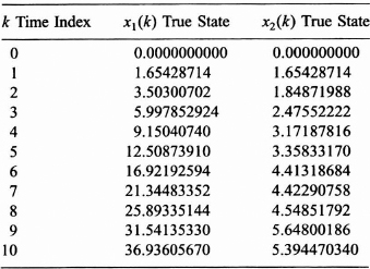
(d) In general, the true values of the state vector are not available. However, for the purpose of illustration the state vector components are given in Tables P8.1 and P8.2. Plot the true values and the estimates for x1(k) determined in (c) on the same graph for k = 1, 2, …, 10. Repeat for x2(k) and its estimate. Compute and plot on separate graphs the error, xi(k) − ![]() i(k|k) for each component i = 1, 2 as k goes from 1 to 10.
i(k|k) for each component i = 1, 2 as k goes from 1 to 10.
(e) Using the error covariance matrix for the state determined by the Kalman filter, as k goes from 1 to 10, plot ![]() and
and ![]() , where ε1(k|k)] = x1(k) −
, where ε1(k|k)] = x1(k) − ![]() 1(k|k) and ε2(k|k) = x2(k) −
1(k|k) and ε2(k|k) = x2(k) − ![]() 2(k|k).
2(k|k).
(f) Comment on the relationship between your errors of part (d) and the variances of part (e).
8.2 In this problem the fixed interval smoothed estimates of the state vector are required using the data and results from Problem 8.1.
TABLE P8.1 Measurement values for Problems 8.1 through 8.3
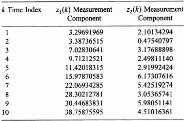
TABLE P8.2 Actual states from simulation for problems 8.1 through 8.3
(a) Compute the fixed interval smoothed estimates ![]() (k|N) for k = 1 to 10, where N = 10, and plot.
(k|N) for k = 1 to 10, where N = 10, and plot.
(b) Compute and plot ![]() (k|10) for k = 1 to 10. Compare your results with those of 8.1(d). Comment on the results.
(k|10) for k = 1 to 10. Compare your results with those of 8.1(d). Comment on the results.
(c) Determine the error covariance matrices for the fixed interval smoothed estimates of the state for k = 1 to 10, and compare the results with those determined in part (b). Comment on the statistical regularity.
(d) What do the off-diagonal terms of the covariance matrix tell us about our estimates?
8.3 We desire ![]() (5|k), the running predicted estimate of x(5), as k goes from 0 to 4, and then the filtered estimate,
(5|k), the running predicted estimate of x(5), as k goes from 0 to 4, and then the filtered estimate, ![]() (5|5), followed by the fixed point smoothed estimate
(5|5), followed by the fixed point smoothed estimate ![]() (5|k) as k varies from 6 to 10. Use the data and results from Problems 8.1 and 8.2.
(5|k) as k varies from 6 to 10. Use the data and results from Problems 8.1 and 8.2.
(a) Compute ![]() (5|k) for k = 1 to 10, and plot each component as a function of k. Indicate on your plots with a dotted line the actual state value for all k (use actual data given).
(5|k) for k = 1 to 10, and plot each component as a function of k. Indicate on your plots with a dotted line the actual state value for all k (use actual data given).
(b) Compute and plot each component of ![]() (5|k) for k = 1 to 10. Discuss your results with reference to the respective error covariance matrix components for the estimate.
(5|k) for k = 1 to 10. Discuss your results with reference to the respective error covariance matrix components for the estimate.
(c) Determine the steady state error covariance matrix for the Kalman filtered estimate of the state vector x(k) defined as
![]()
and discuss the relationship between this matrix and the limited accuracy of the estimation of the state components.
8.4 A system and measurement model for a moving object in a two-dimensional space are given below. The x1(k) and x2(k) could represent the position in an x and y direction at time index k, while x3(k) and x4(k) could represent the velocities in the x and y direction, respectively, at time index k. In the equation the α = 0.97979589.
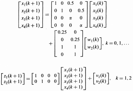
Accordingly, we have the following assumptions:
(1) Initial condition x(0) is a zero mean Gaussian random vector with covariance matrix given as P(0) = 25 I4. Let ![]() (0|0) = [0, 0, 0, 0]T
(0|0) = [0, 0, 0, 0]T
(2) w1(k) and w2(k) are zero mean uncorrelated white Gaussian random sequences with known autocorrelation functions given by
![]()
(3) v1(k + 1) and v2(k + 1) are independent zero mean white Gaussian sequences with the properties
![]()
(4) w1(j) and w2(j) are zero mean and orthogonal to both measurement noise processes v1(k) and v2(k) for all j and k
![]()
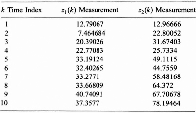
Using the state and measurement models above along with the assumptions specified and Tables P8.4 and P8.5 perform the following tasks:
(a) Use the measurements shown in the tables along with your generated K(k) of the Kalman filter to estimate the current states of the system for k = 1, 2, …, 10. This will give you estimates of the position (![]() 1(k|k) and (
1(k|k) and (![]() 2(k|k) and the velocity (
2(k|k) and the velocity (![]() 3(k|k)) and
3(k|k)) and ![]() 4(k|k)) in each direction from the measurement data.
4(k|k)) in each direction from the measurement data.
(b) Plot the actual position in a reduced state space (two dimensions) from the information on the data and the estimated position on the same plot. (Ordinarily you do not have access to the true location.)
(c) Plot each of the following position errors for k = 1, 2, …, 10.
![]()
These plots give the position estimate errors for your data.
(d) Compare the magnitude of the error at each point for k = 1, 2, …, 10 with the corresponding entry in the error covariance matrix and comment on statistical regularity.
(e) Plot the estimates of the velocities in each direction. (Note that even though the velocities were not measured directly, you are able to estimate them.)
TABLE P8.4 Measurements for Problem 8.4 and 8.5
8.5 Using the models, assumptions, data, and results from Problem 8.4
(a) Obtain ![]() (6|k), k = 0, 1, …, 8. Plot
(6|k), k = 0, 1, …, 8. Plot ![]() 1(6|k) and
1(6|k) and ![]() 2(6|k) for k = 0, 1, …, 8 showing the actual states x1(6) and x2(6) as dotted line for all k.
2(6|k) for k = 0, 1, …, 8 showing the actual states x1(6) and x2(6) as dotted line for all k.
(b) Would you expect your estimate ![]() 1(6|3) or your estimate
1(6|3) or your estimate ![]() 1(6|8) to be a more reliable estimate of x1(6)? Back up your answer by referring to properties of the error covariance matrices.
1(6|8) to be a more reliable estimate of x1(6)? Back up your answer by referring to properties of the error covariance matrices.
TABLE P8.5 Actual state components x(k) for Problems 8.4 and 8.5

REFERENCES
1. Meditch, J. S., Stochastic Optimal Linear Estimation and Control, McGraw-Hill, 1969.
2. Mendel, Jerry M., Discrete Techniques of Parameter Estimation, Dekker, 1973.
3. Kailath, T., Lectures on Linear Least-Squares Estimation, Springer 1976.
4. Anderson, Brian D. O. and John B. Moore, Optimal Filtering, Prentice-Hall, 1979.
5. Sage, Andrew P., and James L. Melsa, Estimation Theory with Applications to Communications and Control, McGraw-Hill, 1971.
6. Srinath, M. D, P. K. Rajasekaran, and R. Viswanathan, Statistical Signal Processing with Applications, Prentice-Hall, 1996.
7. Brown, Robert Grover, and Patrick Y. C. Hwang, Introduction to Random Signals and Applied Kalman Filtering, 2nd Ed., Wiley, 1992.
8. Mendel, Jerry M., Lessons in Digital Estimation Theory, Prentice-Hall, 1987.
9. Candy, James V., Signal Processing the Model-Based Approach, McGraw-Hill, 1986.
10. Brown, Robert Grover, Introduction to Random Signal Analysis and Kalman Filtering, Wiley, 1983.
11. Gupta, S. C., Transform and State Variable Methods in Linear Systems, Wiley, 1966.
12. Cadzow, James A., and H. R. Martens, Discrete-Time Computer Control Systems, Prentice-Hall, 1970.
13. Kalman, R. E. and R. S. Bucy, ‘New results in linear filtering and prediction theory’, Transactions of the ASME Journal of Basic Engineering., Vol. 83, 1961, p. 95.
14. Kalman, R. E., A new approach to linear filtering and prediction problems, ASME Journal of Basic Engineering, March 1960, pp. 35–45.
15. Gelb, Arthur, Ed., Applied Optimal Estimation, MIT Press, 1975.
16. Van Trees, H. L., Detection, Estimation and Modulation Theory, Vol. 1, Wiley, 1968.