
3
Risk Management
3.1. Insurance of risks and risk of insurance
3.1.1. Introductory remarks
One of the principal instruments of risk management is insurance of risks. In fact, it cannot change the risk characteristics (other action is needed for this); however, it can smoothen its different (especially economic) consequences. There are some financial institutions dedicated to this – insurance companies, which compensate (partially or fully) damages that result from the occurrence of risk events. Insurance companies create and possess some special funds for this purpose. This fund consists of the initial capital of the company, insureds’ (individuals or legal entity policyholders) payments (premiums) as a compensation for the transfer of some parts of risks to the insurer, as well as of the financial activity of the company. Thus, the insurer takes onto himself (partially or fully) the risk of the insured, as a result of which the risk of the insurer occurs.
One of the most important parts of risk theory deals with this type of risk; thus, this section is devoted to the description of this type of risk. This study is based on financial mathematics. Here we consider the basic notions and terms of actuarial and financial mathematics, in order to be independent of the special literature.
3.1.2. Basic notions
Actuarial science and practice takes an honorable place in contemporary investigations and education. One of its components (combined with economical and juridical disciplines) is actuarial mathematics. To avoid confusion, based on [BOW 86, DAY 94], some principal notions and terms that are commonly used in actuarial science and practice are defined below.
An insurer is a company that has permission for the fulfillment of insurance activity that undertakes the obligation to partially or fully compensate the insured for the damages if the risk event occurs.
An insurant or policyholder is a person or corporate entity who concludes an insurance agreement.
An insured is a physical or juridical person to whose favor an insurance agreement is concluded.
Insurance rules is a document that determines the general conditions of the insurance company’s activity.
Insurance contract or agreement is a juridical document that concertizes the insurance rules and determines the partners’ obligations and payment premium and benefit conditions in the case of an insurance event occurrence.
Insurance events is a risk event that is marked in the insurance agreement, as an event that leads to the fulfillment of the insurer’s obligations for the benefit payment.
Premium is the payment of an insured in favor of the insurer as a compensation for the transferring his parts of his risk.
Benefit is the insurance compensation that the insurer pays to the insured if the insurance event occurs. The benefit B serves for the damage compensation of the insured. It is not usually equal to damage directly, and it is determined with insurance agreement. Some principles of the benefit calculation will be considered later.
Insurance claim or simply claim is a demand from the insured to the insurer for the benefit payment to the insured or to his legal successor if the insurance event occurs.
3.1.3. Risk insurance models
The risk insurance procedure demands to evaluate both the time to the occurrence of risk event and the value of damage generated by it. The value of possible damage is partially determined by the insurance agreement. With respect to evaluation time to the occurrence of insurance event, insurance models usually follow the risk models and are divided into:
- – short-time insurance models;
- – middle-time insurance models;
- – long-time insurance models.
Short-time insurance models are characterized by the fact that, on the one hand, the insurance event occurs with a small probability and may not occur at all during the insurance agreement period, while on the other hand, inflation processes during this period may not essentially have an influence on the return of the insurer from the premium of the insured.
In the middle-time models, the probability of the absence of the insurance event is also positive; however, the inflation and the interest rate during the contract duration play an essential role in the financial activity of the insurer.
Finally, the long-time insurance models are characterized by the fact that the insurance event occurs with a probability of one, and for the premium evaluation, the inflation processes have to be taken into account at the time of insurance agreement signing.
Each insurance agreement is characterized with some values. Here we consider the following main values:
- – each agreement is entered for some duration time, which will be denoted by T. It could be (i) finite and fixed, (ii) random, up to insurance event occurrence, or (iii) infinite;
- – each agreement provides with the value and order of benefit payments. The value of benefit B can also be fixed or random, depending on the value of damage;
- – each agreement provides with the value and order of premium p payments;
- – besides that the insurance agreement usually provides also for different additional conditions, for example, age of the insured under life insurance or percent equipment depreciation under the floats, planes or other equipment insurance.
For the calculation of these values, we should use the information about the distribution of insurance event time occurrence or about the probability of its occurrence for the case of short-time insurance, and also about the possible damage value distribution in order to evaluate benefit and premium conditions. Therefore, in insurance models, stochastic and some special methods of financial mathematics are very important. They will be considered in the next section. However, we now consider the principal problems that usually arise in insurance mathematics.
3.1.4. Basic risk insurance problems
The insurance process implies that the insurer takes for himself part of the insured’s risks, as well as the obligations for financial compensation of his damages. To do this, the insurer has to have some capital. Because the premium is usually less than the compensation (due to small probability risk or long time to risk event), the insurer usually plays the role of the investor, who invests the insured’s capital into the activity of industrial companies, stocks or state bonds or other securities. The questions about needed reserve (part of the capital that should be rest for benefit payment) is one of the actuarial mathematics problems. The problem of the insurer’s initial capital needed for its stable operation is also closely connected with this problem.
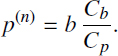
On the one hand, one of the principal problems that any insurer and the state insurance control institutions must consider is the determination of the values and conditions for premium payments for given types of insurance agreements. The problem of the premium calculation is complicated. For its calculation, we should take into account many factors: the insurance event probabilities, the value of possible damages and their different fluctuations, connections with other risks of the insurer, insurer’s expenditure, relation between demands and offers on the insurance market. All these problems are the topics for concrete insurance contracts preparation, and this is not the subject of this book. Therefore, we will focus only on the main ideas of the premium calculation. The premium p is usually divided into two parts: net-premium p(n) and insurance load p(s).
The net-premium p(n) serves to cover the basic insurer’s expenses. Its calculation is based on the equivalence of financial obligations principle, which means the equity of insurer and insured payments in mean and require that the net premiums will be equal to the mean value of the benefit. The insurance load p(s) provides stability of the insurance company that is represented as the negligibly small probability of its ruin.
Thus, the principal problems of actuarial mathematics (and practice) are an elaboration of methods for:
- – estimation of the time to risk (insurance) event distribution (or its parameters), probability of this event occurrence for short-time risk models;
- – estimation of the damage value distribution (or its parameters);
- – initial capital and reserves of insurance company determination;
- – insurance premiums (net premium and insurance load) calculation;
- – value and order of the premium payment.
For the solution of these problems, a detailed study of insurance agreements is needed, which is the goal of concrete insurance rules and agreements elaboration. Moreover, in the next section only some simple illustrative examples of risk insurance mentioned in section 2.1.2 will be considered.
3.1.5. Examples
Consider some very popular insurance examples and some other examples that might not be realized up until now, but could be of interest in the future.
EXAMPLE 3.1 Life insurance.– Life insurance is not only known as endowment insurance or death insurance (this type of life insurance is known as whole life insurance), but also as the insurance for the case of different situations connected with the person’s life. An example of a short-time life insurance is considered below. Suppose that the duration of an insurance agreement is one year T = 1, for the insured aged x years and the insurance agreement stipulates three risk events:
- – death of the insured does not occur during the insurance agreement time period with the nothing compensation b0 = 0;
- – the “natural” death of the insured occurs during the agreement time period with the fixed benefit b1 payment;
- – the insured death resulting from an accident with the fixed benefit to his/her legal successor of the value b2 payment.
For this model, the problem of the insurer involves the determination of the premium value p that will provide a fair payment for the risk, accepted by the insurer. The solution of the problem will be presented as Examples 3.8, 3.10 in sections 3.3.2 and 3.3.6.
EXAMPLE 3.2 Property insurance.– Consider now the property risk insurance connected, say, with an auto accident during the agreement time T = 1 year and uniformly distributed in the interval [$ 100, $ 2000] value of damage in the case of risk event occurrence. Furthermore, the task of the fair insurance premium calculation is also solved as Examples 3.9, 3.10 in sections 3.3.2 and 3.3.6.
EXAMPLE 3.3 Insurance against industrial injuries.– Industrial injuries are a serious social and economical problem. The consequences of these injuries could be partially smoothed by some efficiently organized system of the insurance against this type of risk events. Consider some simplified scheme of this type of insurance. As insured here might be the collaborator of some enterprise or the enterprise itself, which insures its collaborators in order to ease the burden of damages if the risk event occurs. As an insurance event here we could consider:
- – an individual accident, which leads to the death or partial/full loss of workability to one separate worker;
- – an accident, which leads to the death or partial/full loss of workability to some group of workers;
- – ends of the insurance agreement without any insurance event occurrence.
The problems of the risk event probabilities, the number of injured workers as well as values and order of benefit and premium payments are specific for each enterprise and should be proposed as a result of special statistical and economical analysis.
EXAMPLE 3.4 Oil well insurance against depletion [RYK 98].– According to the US statistical data, approximately 10–15% of US oil production is carried out from low-debit oil wells (a low debit well produces less than 10 barrels per day). In Russia, there are many oil wells with small debit, which, unfortunately, under the condition of different economical reasons became unprofitable and are now closed. Except for economical losses, this also leads to some social tensions. In order to prolong exploitation of low-debit wells and fields and provide profitability, we should use well insurance against depletion, which could be used as an economical instrument for the productivity support of wells and field areas.
The substance of such insurance consists of the creation of a special fund that during profitable well exploitation (with normal debit) will collect some capital as premium deduction and use it for prolonged periods of low-debit wells. The facilities of this fund could be used for tax payment, financing of social expenses, etc. The problems of conditions, rules, and models of actuarial calculations arise for this type of insurance. The simplest model of such type of insurance looks like a pension fund model and consists of the following.
The field area owner during the well time exploitation T1 with debit Q > Q* from the the time t0 puts into operation and up to the time t0 + T1 decreases the debit up to level Q*, and pays periodically the premium p with fixed interval (for example, once per year, quarter or month) to the insurer for special “Fund” creation, and the insurer agrees to pay the insured (field owner) benefit as payments of the size b after the time t0 + T1, when its debit becomes less than Q*, up to the time t0 + T of its full decommissioning. The benefit could also pay periodically (say also, once per year, quarter or month). It is assumed that if the well will be closed for any reason before its debit decreasing below the level Q*, then the accumulated premium amount to this time will be returned as accumulated benefit or used as a compensation for another well. Thus, three types of insurance events are considered:
- – the well debit falls below the level Q*; in this case the periodical payment of premium stops, and the insurer became pay benefits;
- – the well is closed for some reason before its debit falls below the level Q*; in this case, the payments of the premium stop, and the accumulated premium amount is returned to the insured as a cumulative benefit or is used for other benefit payment;
- – the well is closed after some time T of its full decommissioning, and then the insurer stops the benefit payment.
We now consider the example given in section 3.3.2.
EXAMPLE 3.5 Ecological insurance.– The necessity of ecological insurance is evident to specialists, and today there exists some progress in this direction. However, this type of insurance organization is restricted by several factors:
- – absence of probabilistic models about the origin and evolution of ecological disasters and catastrophes;
- – absence of sufficient statistical data about these types of risks;
- – absence of juridical base needed for this type of insurance organization.
Nevertheless, consider some rough models for ecological insurance, which could be useful for this type of insurance organization.
Suppose that the owner of an oil or gas pipeline, nuclear power station, chemical or other dangerous enterprise, or administration of some seismic, or other ecologically dangerous regions make an agreement with some insurer on partial or full compensation of damages of industrial objects, personal properties, etc. that result from ecological disasters. The risk events with serious ecological consequences should be considered here as the insurance events. They should be differentiated both by their types and possible damage. The premium amounts are paid regularly with fixed periodicity from the enterprises with high ecological hazard or ecologically dangerous region budget, and the benefits are paid by the insurer in the size of damage value or according to the contract conditions if the insurance event arises. The initial data needed are:
- – distribution time for insurance event occurrence, or at least its parameters;
- – damage value distribution; or at least its parameters.
The data obtained is a subject of serious statistical and economical analysis. Different kinds of models with different periods and sizes of premiums and benefits can be investigated to choose the best one.
EXAMPLE 3.6 Educational insurance.– In many countries, education is expensive and beyond the financial means of some families. However, these families often have the best prospects in terms of the return on money spent on education.
Moreover, under conditions of quick development of technological processes, knowledge and skills become obsolete fairly quickly, which leads to the necessity of training various levels of employees. For these problems, some type of insurance in the sphere of education and training will also be helpful. Some model examples of this kind of insurance are given below. Insurance considers the following events:
- – attainment by the insured of a usual school age;
- – beginning of the education in special or high school, or university;
- – loss of workability or working place and the training needs;
- – during the contract time none of these events occurs.
Analogously to the previous example, the premium amounts of the given size are periodically paid to the insurer, and the benefits are also periodically paid for the school, university or other educational institution. If none of the above events occur during the contract time, the benefit is paid at the end of the agreement time. The calculation of the appropriate characteristics of this type of insurance is a problem of this type of insurance development.
These examples will be further used for the illustration of insurance characteristic calculation methods. However, most of these methods (especially for long-time insurance models) are based on financial mathematical methods. In the next section some basic notions and methods of financial mathematics will be discussed briefly.
3.1.6. Exercises
EXERCISE 3.1.– Write the initial parameters and the searching characteristics for the insurance models given in the above examples.
3.2. Some notions and methods of financial mathematics
The insurer usually uses accumulated premiums of the insured for investments, as mentioned previously. Therefore, the insurer acts as an investor and its financial operations should be taken into account for the above formulated solution of problems. Appropriate problems are usually considered in the framework of financial mathematics. Thus, this section deals with some principal notions and methods of financial mathematics according to [LYU 02, PAN 01, MAC 02].
3.2.1. Principal notion of financial mathematics
Financial mathematics studies different financial operations, the simplest of which is the credit operation. The latter consists of rendering monetary or other facilities from one corporate entity or individual to another according to some contract credit agreement. The basic subjects (corporate entity or individual) of financial activity are lenders (investors) and borrowers (debtors). A lender (investor) is an entity or individual who gives the facilities (usually money) to another entity or individual borrower (debtor) according to the credit agreement.
Note that concerning the insurance agreements, the same “subject” in different operations can play different roles. Especially in the insurance agreement, the insured plays a role of a creditor and the insurer plays the role of a borrower. However, during the management of the capital and putting the activities of the company in different projects or other activities, the insurer acts as an investor before other debtors.
The following parameters determine the credit operations:
- – the time t0 of the agreement conclusion;
- – duration T of the agreement (for insurance, agreements that are distinguished by it from the usual credit operations, in which the agreement duration is usually fixed, while in long-time insurance agreements, this period is random);
- – time t0 + T of agreement completion (fulfillment of contract obligation).
Denote by S (t0) the value of credit (for insurance agreements, this is the value p of premium) and by I(t0, T, p) the loan payment (the value of increment during the insurance agreement time). Then the value
is the full credit price, or in the terminology of insurance agreements, it is the benefit.
It is well known that the price of money changes over time, and one of the most important problems of financial mathematics is to find the present value (PV) of the future sum of money. It is known as discounting, and the appropriate coefficient is called the discount factor. Thus, the following values that naturally depend on all of the above parameters are: the time t0 of the contract conclusion, the duration T of the contract, and the value of credit S (t0) (premium p for insurance agreements). These values can be used for the calculation of credit operations:
- – interest rate, return,
[3.1]
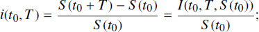
- – discount rate,
[3.2]
- – discount factor,
[3.3]
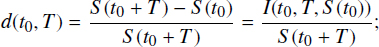
Because the contract durations are different, and the benefits are random, for unification of the returns for different contracts, it is necessary to consider some basic period for it; such a period is usually expressed as one year in financial mathematics. Taking into account a basic period of one year, T = 1, and omitting other contract parameters, put
It is not difficult to check whether a closed connection exists between these values,
These connections allow us to calculate any two indexes if one of them is known. Due to this, from the mathematical point of view, it will be enough to operate with only one of these indexes. However, the financial practice in different situations uses different indexes, and we will follow this practice.
As mentioned above, the price of money changes over time, and this variation is represented in terms of interest rate. Consider two main principles of the change in money price.
3.2.2. Simple interests
According to the simple interest principle, accruals are produced only for the basic endowments. For any basic period, the formula for accrued endowment during T = n periods under the constant interest rate i takes the form
We know (see exercise 3.5) that for a constant interest rate i the sequence of accruals for n period sums forms an arithmetic progression with the initial term a0 = S (t0) and the difference iS (t0).
As mentioned above, one of the most important characteristics of the financial operation is the present value of the future sum of money. According to [3.5] in order to get at time t0 + T the sum of money S(t0 + T) under the constant interest rate i(t0), it is necessary to put in time t0 the sum

Thus, the value
is called the discount factor and the difference
is called discount.
Let us consider two more important questions connected with the endowment accumulation under simple interest: variable simple interest and the return investments under simple interest. If during the term of the agreement the simple interest rate is changed, then the procedure of interest accrual is called the variable interest. Let us now consider the process of the endowment accumulation in this case. During the contract time [t0, tn], let the interest be changed in epochs,
and it remains a constant equal to ik inside the intervals (tk−1, tk]. Then it is not difficult to calculate that up to epoch tn and thus the accrued endowment will be equal to

The initial value of endowment is increased to the value
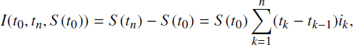
and the accrued factor will be

Let the accrued with the simple interest to each of the epochs tk return be invested for the next period (tk, tk+1], i.e. the accrued to the time t1, capital is invested under the simple interest i1 to the next period (t1, t2]. Then the accrued to the time tn capital will be equal to

The more complicated procedure of the capital accumulation is realized when the compound interest is used.
3.2.3. Compound interests
According to the compound interest principle, the accruals are realized not only to the basic capital, but also to get its interest. Thus, the procedure of accruals under compound interest coincides with the procedure of accruals under simple interest with reinvestments for the case of constant reinvestment period and interest. The value of the basic period becomes more important because the formula of the accumulated capital takes the form
where i is the interest for the basic period τ = 1, and n is the number of basic periods during the term of agreement. From this formula, it follows that the capital accrued under compound interest forms geometric progression with the first term b1 = S (t0) and denominator q = (1 + i) (see exercise 3.8).
Thus, we can see that when credit is given under simple interest, then the accumulated capital increases linearly and the period of accrual in this case does not play an essential role, but in the case of compound interest, the accumulated capital increases as a geometric progression and the accrual period becomes more important in this case. This is shown by an example.
EXAMPLE 3.7.– Let $ 100 000 be given for two years under a 100% interest rate per year with accrual once per year and twice per year. Then the accrued sum of capital in the first case will be
and in the second case, it will be
It is possible to see that the difference is essential.
Let us consider the interest accrual period in more detail.
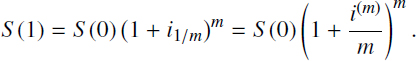
DEFINITION 3.1.– Yearly interest rate is called nominal for the accrual period 1/m and is denoted as i(m) if it is equal to m-multiple rate of this period, i.e.
Therefore, accumulated capital for the basic period (year) will be
It is evident that when m increases, then the accumulation factor
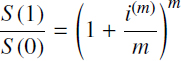
also increases. With the increasing frequency m and the decreasing interest accrual period, we get the model of continuous accrual of interest. It is clear that with the increase of the frequency interest accrual m the nominal year interest rate i(m) has to have a limit, which is denoted by δ and is called the intensity of accumulation or nominal year interest rate for continuous compounding.
DEFINITION 3.2.– Effective year interest rate is called the rate i that provides the same accumulation as the continuous rate.
Thus, from this definition and due to the limiting relation
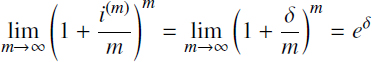
it follows that
Analogous to the case of simple interest, the inverse problem about the required value of investment under the effective compound interest rate i in order to get the required sum of capital S (t0 + t) at a given time t0 + t can be solved. From the formula [3.11] we have

which for continuous interest accrual gives
The operation for finding the needed value of investment (deposit) in order to get the given value of the capital at a given time is called discounting), and the appropriate coefficient is known as the discount factor. Thus, the effective year discount factor is determined by the formula ![]() , and the continuous discount rate is given by e-δ; and the value δ is the discount intensity, as defined previously.
, and the continuous discount rate is given by e-δ; and the value δ is the discount intensity, as defined previously.
Note that according to the insurance agreement, the premium can be paid as a one-time payment in the time of contract opening, or according to the contract conditions as a flow of payments. The task of the insurer (and actuarial mathematics) consists of the calculation of the payment flow parameters in order to provide the benefit payment at the time of contract completion.
3.2.4. Cash flows and the financial rents
Many financial operations (including those under insurance agreements) assume not only a one-time payment but also periodical payments (premiums and benefits). This type of financial operation is known as a cash flow. Any cash flow π is determines with times tj of payments, which is ordered in increasing manner,
and their values zj.
DEFINITION 3.3.– The sequence
with two-dimensional values (tj, zj), where tj are ordered times of payment, and zj are their values, is called cash flow. The payments will differ for positive and negative, denoting the positive by xj and negative by yj, zj = xj – yj (j = 0, 1,…).
The principal problem of investigation and comparison of the cash flows is solved by their reduction to the same point in time. The general model for cash flow comparison consists of the following. If t0 is the time of contract conclusion (signing, beginning, not completion) and the payments of sizes zj are paid in times ![]() , then at the time tn of contract completion, the capital will be equal to
, then at the time tn of contract completion, the capital will be equal to
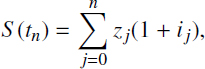
where ij = i(tj, tn) is the interest rate during the period (tj, tn).
The principal characteristic of the cash flow is its present value (PV), i.e. its price calculated at the time of contract conclusion. Taking into account the change in the money cost in time for the present value of incomes and consumptions, the relations hold
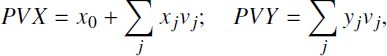
where vj is the discount factor at the period (t0, tj].
The most common forms of cash flow in financial mathematics are the financial rents.
DEFINITION 3.4.– The cash flow with the constant rate of return and positive payments that is realized after the same time intervals are called financial rent or annuity.
From the definition, it is clear that the rent is determined by the rate of return i, period τ = tk – tk-1 of payments and the members of rent zk = xk.
DEFINITION 3.5.– The rent is termed constant if all of its members are equal xk = x, otherwise, the rent is known as variable.
The duration of the rent T is usually multiple to its period τ and equal to the number of payments n by the period, T = nτ. In theoretical analysis, it is convenient to put τ = 1, so T = n. For rent analysis an essential role is played by the relations between the period of interest accrual, payments period and basic period.
DEFINITION 3.6.– Taking a year as the basic period, define the discrete (l, m) - fold rent as a rent in which payment is realized l times per year, and the interest is produced m times per year.
The rent is called an ordinary one if the accrual and payments periods coincide l = m; otherwise, the rent is called general. If the payments and accruals are performed too often, for example every day or more often, then it is advisable to analyze them as a continuous one. Such rents are called continuous.
An essential role is also played by the rule of payments in discrete rents: at the beginning or at the end of each period.
DEFINITION 3.7.– If the payments are performed at the beginning of each period, the rent is called proactive annuity or advance annuity; if they are performed at the end of each period, it is known as retarded or regular annuity.
Other cases are also possible. Pension payments, when paid in some fixed days, could be an example of such a kind of rent. This kind of rent will not be considered here because its characteristics take the values between the advance and regular annuities.
From the point of view of annuity duration, they are divided into unconditional annuity and imputed rent. For the first one, the times of the beginning and end of payments are fixed; for the second one, the times of one or both can be random and can depend on some additional events. For risk insurance, we usually deal with imputed rents.
DEFINITION 3.8.– An annuity is called perpetual if it has an infinite duration. An annuity is called deferred for the time t1 if the payments for it begin after the time t1 of a contract opening, or from the time t0 + t1.
Consider the principal indexes of the ordinary annuity, using standard for the financial mathematics notations. It is clear that for the calculation of annuities PV, the most essential role is played by the accrual and discount factors. The indexes will be considered for the rents with single payment because for the payment of arbitrary size, they are obtained by a simple multiplication. The appropriate indexes are shown for advance and regular annuity.
The PV to time of the contract completion of an advance annuity is equal to
The PV to time of the contract completion of an regular annuity equals, respectively,
From these formulas, it is possible to express the accumulated cost of rents to the time tn = n of the contract completion in terms of their cost at the initial time t0 = 0. According to [3.4] and [3.11] from the formulas [3.16] and [3.17], respectively, we have
Therefore, the accumulation factors for the advance and regular annuities, usually for financial mathematics notations, equal, respectively,
and discount factors are
In the following two sections different risk insurance models will be considered in more detail, and this section, as always, ends with exercises.
3.2.5. Exercises
EXERCISE 3.2.– Using formulas [3.4], calculate discount rates and discount factors for the yearly interest rates i = 2%, 5%, 10%, 20%, 50%, 75%, 100%.
EXERCISE 3.3.– Calculate the yearly interest rates and discount factors for the given discount rates d = 2%, 5%, 10%, 20%, 50%, 75%, 100%.
EXERCISE 3.4.– Calculate discount rates and yearly interest rates for given discount factors v = 2%, 5%, 10%, 20%, 50%, 75%, 100%.
EXERCISE 3.5.– Prove that under a simple constant interest rate i the sequence of accrued sums during n periods forms an arithmetic progression with the initial term a0 = S (t0) and the difference d = i.
EXERCISE 3.6.– Prove the formulas [3.7]–[3.9] by induction.
EXERCISE 3.7.– Prove the formula [3.10] by induction.
EXERCISE 3.8.– Prove that under a compound constant interest i the sequence of accrued sums during n periods forms a geometric progression with the initial term a0 = S (t0) and the denominator q = 1 + i.
EXERCISE 3.9.– Find the required credit sum for 9 months under the compound interest at 60% per year with the condition to return $2 million.
EXERCISE 3.10.– Prove that the discount rate d for the credit contract that is equivalent to the yearly interest rate i equals to ![]() This value is called the annual discount rate.
This value is called the annual discount rate.
EXERCISE 3.11.– Calculate the size of debt for credit of $500 given for the half of year under the compound interest 10% per month.
EXERCISE 3.12.– Calculate the value of credit for 2 years under the compound interest 15% in quarter, the return for which equals to $ 1.2 million.
EXERCISE 3.13.– Calculate the accrued sum and increments of the capital from 2 years credit under the compound interest i% per year when it charges:
- – annually,
- – biannually,
- – quarterly,
- – monthly,
- – weekly,
- – daily (if the year contains 365 days).
Represent results in a table.
EXERCISE 3.14.– Calculate the period of the capital doubling in the credit agreement under compound interests i = 5%, 10%, 25%, 50%, 75%, 100% per year. Represent results in a table.
EXERCISE 3.15.– Calculate the discount factors and provisions for permanent simple proactive and delayed rents for periods n = 1,2,…, 10 at different rates i = 2%, 5%, 10%, 25%,50%.
3.3. Short-time insurance model investigation
3.3.1. Introductory remarks
The typical examples of short-time insurance models are:
- – annual insurance of dangerous enterprise collaborators against accidents,
- – annual vehicle insurance against accident or stealing,
- – annual house and other property insurance against fair and other accidents,
- – train, aircraft and boat passenger insurance during traveling,
- – athlete insurance from injury during competitions, etc.
The short-time insurance risk models are characterized by the small value of the risk event probability, on the one hand, and by the possibility of not taking into account the inflation process, on the other hand. The tasks of insurers is to estimate the risk event probability, study the possible damages, calculate the premium value needed for their compensation and provide the stable operation of the insurance company. The tasks of the state insurance supervision consists of providing the insured’s interests and limiting excessive profits of insurers.
It is necessary to note that the theoretical study of risk models might be fulfilled independently of the real realization. It gives the possibility of using this study for different applications by engaging concrete data. Let us consider some short-time risk models and examples of their index calculation.
3.3.2. Calculation of the individual claim indexes
For the short-time insurance model study, we will further denote the insurance events by A or by Ai, if the insurance agreement involves several such events, the indicator function of the event Ai by I{Ai}, and by the claim size in the case of the ocurrence of event Ai by Xi. Let us also denote by qi the probability of event Ai, and by μi and ![]() the conditional expectation and variance of the claim value under the condition of the occurrence of insurance event,
the conditional expectation and variance of the claim value under the condition of the occurrence of insurance event,
For the calculation of full damage characteristics, it is very convenient to use the general formulas of complete probabilities and complete expectations, whose calculation of the expectations and variance have the form
For considering the special case Y = IAi, on one hand taking into account that E[X|I = 0] = 0 and E[X|I = 1] = μ, we find E[X|I] = μI. On the other hand because X = 0 for I = 0, so Var[X|I = 0] = 0 and as Var[X|I = 1] = σ2 for I = 1, so Var[X|I] = σ2 I. Thus E[Var[X|I]] = σ2Var[I] = σ2q, and therefore
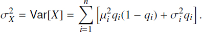
Finally, taking into account that Var[I] = q(1 – q) and then using general formulas [3.25] and [3.26], we find
Analogously to the case of insurance contracts, containing n risk events Ai, or to the portfolio from n contracts with parameters given by the formula [3.24], we have

For the illustration of these formulas in practice, two examples are considered.
EXAMPLE 3.8 Short-time life insurance.– Consider again example 3.1. We assume that the agreement involves the following conditions:
- i) in the case of the insured’s death during the accident, the insurer pays the benefit of the size b1, and;
- ii) he pays the sum b2 in the case of death for another reason1;
- iii) let the probabilities of appropriate events be q1 and q2.
Let the insurance conditions and the age of the insured determine these values as
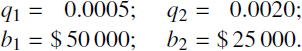
Then, the joint distribution of the insurance event and the insurance compensations take the form

By summing, we find P{I = 1} = 0.0025 and, respectively, P{I = 0} = 0.9975. Furthermore, the expectations and variance of the benefit are

EXAMPLE 3.9 Vehicle accident insurance.– For the model of vehicle accident insurance, we consider example 3.2. Let the probability of accident during an insurance period, say a year, be equal to q = 0.15 and the evaluation of damage (which certainly depends on the vehicle type) has a uniform distribution with step 10 between $ 100 and $ 2000. The conditional means μ and variance σ2 of the benefit in this case according to the characteristics of uniform distribution (see section 2.2.2.2) are
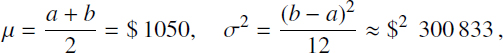
and, therefore, according to the formulas [3.27], its non-conditional means E[X] and variance Var[X] are
3.3.3. Exact calculation of summary claim characteristics
One of the most important problems for the insurer is the calculation of the summary claim distribution from its contract portfolio. Under the assumption of independence of separate contracts (which is quite acceptable for individual insurance), such a calculation is made possible by the convolution of the individual claim distribution. Such a calculation is made for a discrete distribution that is mostly natural for the claim distribution. Assuming that the insurer has concluded n homogeneous contracts, for each of which the claim ![]() has an integer distribution
has an integer distribution
The summary claim
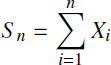
is also an integer-valued r.v., but with higher values than each of the summand. Thus, S2 takes 2m + 1 different values, S3 takes 3m + 1 values, etc. The summary claim Sn of n homogeneous r.v. can take mn = m ᐧ n + 1 different values.
Find the distribution of the summary claim using the complete probability formula. Fix one of the possible values, say k, of r.v. Sn and consider all possible variants different values of r.v.’s Xn, which can lead to the event {Sn = k}. On one hand, if k > mn−1, then Xn can take values not less than k – mn−1. On the other hand for k < mn−1, the value of r.v. Xn cannot be greater than k. Therefore, the r.v. Xn can change their values between and J1 = min{mn−1, k}. With this argument, for ![]() , we obtain
, we obtain
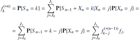
We should begin the calculation from ![]() , and then recursively calculate
, and then recursively calculate ![]() . The formula is known as the discrete convolution formula, as indicated previously. The calculations can be represented with the help of the matrix, whose rows f = [f1, f2,…, fm]ʹ and
. The formula is known as the discrete convolution formula, as indicated previously. The calculations can be represented with the help of the matrix, whose rows f = [f1, f2,…, fm]ʹ and ![]() are the probability vectors of r.v.’s Xn and Sn-1, respectively,
are the probability vectors of r.v.’s Xn and Sn-1, respectively,

to get the value of convolution, we should sum the elements of side diagonals of this matrix.
3.3.4. Normal asymptotic of summary claim distribution
The exact calculation described in the previous section are cumbersome, and really not needed, because for a sufficiently large number n of contracts, the distribution of summary claim Sn due to the central limit theorem of probability theory is very good, approximated with a normal distribution. This theorem has been mentioned before as theorem 1.7 in section 1.2.1.5. Repeat theorem is presented here for the approximation of the summary claim distribution.
THEOREM 3.1.– Central Limit Theorem. If ![]() , then the following limiting relation is true:
, then the following limiting relation is true:

![]()
The values of the function Φ(x) are given in the tables of standard normal distribution or in any computer statistical program packages.
This relation allows enough precise calculations for the necessary probabilities in the case of sufficient values of x (for the case of sufficient values of insurance event probabilities). However, this approximation is not good enough for the “tails” of the normal distribution, i.e. in the case of small insurance event probabilities, which is usual for short-time insurance models. In this case, more appropriate is the Poisson approximation that is specially adapted to Bernoulli (two-valued) distributions.
3.3.5. Poisson asymptotic of summary claim distribution
Consider now the sum Sn of n Bernoulli (two-valued) r.v.’s ![]() ,
,
It is well known that it has the binomial distribution
THEOREM 3.2.– If for n → ∞ and q → 0, the relations nq → λ holds, then the following limit relation holds:
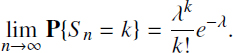
![]()
Of course, in practice, we should use this theorem if n >> 1 and q << 1, where λ takes the value λ = nq.
3.3.6. Calculation of insurance basic characteristics
The problem of the detailed study of all insurance problems is not the subject of this book. Therefore, we will only focus on some of them, especially the problem of the insurance premium calculation. Moreover, due to a wide variety of insurance contract structures, it is quite impossible to consider most of them. Thus, the principles of the premium calculation will be demonstrated with the help of some problems considered in the examples presented in section 3.1.5. As was mentioned above in section 3.1.4, the full insurance premium p consists of two parts: the net-premium p(n) and insurance load p(s). The net-premium serves for the covering of basic insurer’s expenses and its calculation is based on the equity payments principle, which requires that the net premiums will be be equal to the mean value of damage from the insurance event. Thus, for the short-time insurance contract, this principle gives
EXAMPLE 3.10.– For example 3.8, for short-time life insurance, it thus gives p(n) = E[X] = μx = $75. Note that in this case the sides of the insurance contract do not deal with the real damage X, but with its partial compensation, given in the insurance agreement.
Another example 3.9 of vehicle accident insurance is that an appropriate net premium should be equal to p(n) = E[X] = μx = $ 157.5.
The insurance load that serves to provide the stability of the insurance company for providing a negligible probability of its ruin is based on the normal approximation of the summary claim. Here, the ruin means that the accumulated company funds do not cover its expenses. Assuming that the insurer has a sufficiently large number n of homogeneous contracts, calculate the insurance load from the condition of the negligibly small ruin probability of the insurer,
Here the ruin probability means the probability that the summary company expenses (summary benefit) ![]() exceeds the summary premium (p(n) + p(s))n. Taking into account that the net-premium is calculated based on the equivalence principle and equal to the mean benefit, E[Sn] = np(n), for the ruin probability ψ with the help of CLT, we find
exceeds the summary premium (p(n) + p(s))n. Taking into account that the net-premium is calculated based on the equivalence principle and equal to the mean benefit, E[Sn] = np(n), for the ruin probability ψ with the help of CLT, we find
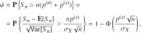
because ![]() Taking the given ε as the appropriate quantile of normal distribution z1-ε, such that the inequality
Taking the given ε as the appropriate quantile of normal distribution z1-ε, such that the inequality
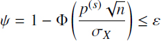
holds or equivalently Φ(z1-ε) ≥ 1 – ε, evaluate the insurance load in the form
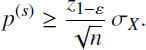
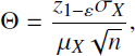
It is very convenient to represent the insurance load as a fraction of the net premium, p(s) = Θp(n). Thus, because of the equivalence principle, the net premium is equal to the mean premium from one contract, p(n) = E[X] = μX; for the insurance load factor Θ, we can find
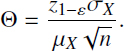
For the rough evaluation of this value, we can use the “3 σ–rule”, according to which the deviation of the normally distributed r.v. from its mean that is more than three standard deviations does not increase to 0.1%. Thus, using this rule, we can find

An analogous result is preserved in the case of enough large portfolios of r groups of ni homogeneous contracts in the i-th group, with damages Xij, ![]() being independent and having different expectations
being independent and having different expectations ![]() and approximately the same variances
and approximately the same variances ![]() In this case, the expectation of the sum of all damages is
In this case, the expectation of the sum of all damages is
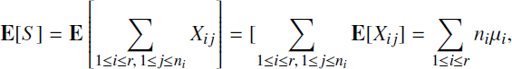
and the variance is
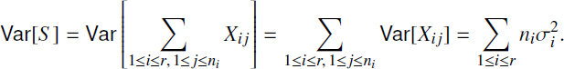
Therefore, denoting by n the whole sum of contracts n = Σ1≤i≤r ni, we can get the same expression [3.31] for the ruin probability evaluation with the same results of the insurance load evaluation. This evaluation shows that the insurance load quickly decreases with the number of contracts of the insurer (or its activity).
In the next section the models of middle- and long-time insurance are considered. These models also use both the probabilistic methods due to the random nature of risk, and financial mathematics methods, because there are possibilities of accumulated investments by the insurer’s endowment.
3.3.7. Exercises
EXERCISE 3.16.– Calculate conditional and unconditional mean values and variances of the insurer’s benefits for the insurance scheme of example 3.8 for your own numerical data of its parameters.
EXERCISE 3.17.– Calculate the exact distribution of the benefits for three customers, whose contracts coincide with the scheme of example 3.8.
EXERCISE 3.18.– Calculate the exact distribution of the benefits for insurance of two vehicles, whose contracts coincide with the scheme of example 3.9.
EXERCISE 3.19.– Using the normal approximation, evaluate the probability that the summary insurer’s compensation for 100 contracts, according to the scheme of example 3.8, and 20 contracts, according to the scheme of example 3.9, increases to $50 000.
EXERCISE 3.20.– Using the Poisson approximation, evaluate the probability that the summary benefit of an insurer who concludes 50 contracts according to the scheme of example 3.8, and 10 contracts according to the scheme of example 3.9, will be greater than $10 000.
3.4. Long-time insurance model investigation
3.4.1. Introductory remarks
Insurance of long-time risk events leads to long-time insurance problem investigation. Examples of long-time risks of insurance models are: ecological and technological risk insurance, full life insurance, pension insurance, etc. Although the long-time risk models suppose the risk event occurrence to have a probability of one it does not mean that the long-time insurance contracts obliges waiting until the insurance event occurrence. It only means that the management of long-time risks has to provide the measures for its prevention. If for some type of models, such as full life insurance or ecological insurance, this is impossible, then for another type of insurance model (transport or some dangerous enterprise insurance) it will be necessary to calculate, for appropriate α, the α-guarantee time of the system operation and therefore to determine their decommissioning period.
If in a short-time risk insurance model, the difference between the premium and benefit is attained due to a small insurance event probability, then in middle- and long-time risk insurance models this difference is attained due to management of the insurer’s endowment during the insurance period. Therefore, the calculation of the parameters of middle- and long-time insurance models is essentially based on (both) the financial mathematics and probability theory methods; while the latter must take into account the random nature of risk. As the methods of middle-time risk insurance are analogous to those for the long-time insurance models, we will limit ourselves to the long-time insurance models, giving some commentaries for the first case.
3.4.2. The basic parameters of long-time insurance contracts
The long-time insurance contracts are characterized by manifold structures and parameters. The basic ones among them are as follows:
- – Contract conclusion time t0; for theoretical calculations, it can be taken as zero, t0 = 0.
- – Contract duration T = T(t0, x); this value can depend on the contract conclusion time t0, as well as on any other parameters, for example age x of the insured for life insurance, or equipment depreciation x for technological insurance, etc.
- – Time T1 = T1(t0) to insurance event occurrence; usually this time is the residual time to the insurance event occurrence from the time t0 of insurance.
- – Combined with times T and T1, it is convenient to consider two other connected values:
- - time to ending of the premium payment,
- - duration of the insurance rent (benefit payment),

- - time to ending of the premium payment,
- – Value of the benefit payment; here, there are different cases:
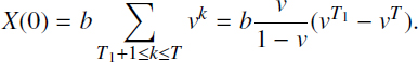
- - random lump sum B benefit payment in the time T1 of the insurance event occurrence (usually it takes place with some delay; however, we will omit this). The summary reduced to the time of contract opening benefit value X(t0) will be equal to
where i = eδ – 1 is effective annual interest rate, δ is the interest intensity, and v = 1/(1 + i) is discount factor;
- - random lump sum B benefit payment in the time T if the insurance event does not occur before the time of contract completion. The summary benefit will be equal to

- - fixed benefit b(ti) payments in times ti (T1 = t1 ≤ t2 ≤ … ti ≤ … tN = T) during the period [T1, T] if an insurance event occurs in time T1; then the PV to time T0 summary benefit will be equal to
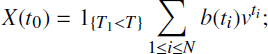
- - fixed benefit b(ti) payments in times ti up to infinity (in spite of the seeming impossibility of such types of contracts, they can in fact take place). It is also possible to assume that the insurer agrees to pay the benefit for the consequences of some ecological catastrophes “infinitely” with the transfer of obtaining rights by inheritance or by saving these rights.
- - random lump sum B benefit payment in the time T1 of the insurance event occurrence (usually it takes place with some delay; however, we will omit this). The summary reduced to the time of contract opening benefit value X(t0) will be equal to
- – Premium value can be paid:
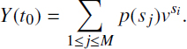
- - as a fixed lump sum p in time t0 of the contract opening, thus the PV premium equals to Y(t0) = b; or
- - as a fixed value p(sj) in sj (t0 = s1 ≤ s2 ≤ … sj ≤ … sM = T1) up to time T1 of an insurance event occurrence, thus the PV to time t0 summary benefit will be equal to
Of course, we should take into account that these values are r.v.’s, which are determined with their distributions. As it will be seen later for actuarial calculations, it will often be enough to limit ourselves to their two moments. As the premium and benefits are usually distributed in time, they represent some special case of financial rents, and we briefly consider their peculiarities.
3.4.3. Insurance annuity analysis
Note first that the insurance annuity differs from the usual financial annuities due to the randomness of most factors involved: contract duration and the times of beginning and ending payments of insurance premiums and benefits as well as the value of damage, which determine the value of the benefit payment. These facts seriously complicate the calculation of all indexes of insurance contracts and the company operation.
It is not the goal of this book to give the analysis of all possible schemes of risk event insurance. Here, we demonstrate some problems of this type of insurance with the simple scheme insurance annuity analysis. Thus, the annuity analysis for insurance contracts will be demonstrated for the case of periodic payments of insurance premiums and benefits. The numerical illustration of this analysis will be presented in section 3.4.6 for an artificial example 3.4 of oil wells from depletion insurance. For convenience, the time will be measured in units divisible by the period of benefit and premium payments, which is also supposed to coincide with the period of interest accrual. Moreover, according to the assumption presented in section 3.2, the annuities with different signs will be considered separately and only the case of fixed benefits and premiums will be considered, and for theoretical calculations, the contract conclusion time t0 can be taken as zero, t0 = 0.
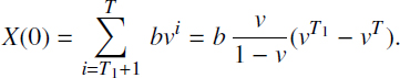
Suppose that both premiums and benefits payments are carried out with the same periodicity, say once a year, a quarter or a month (although it is not too difficult to realize the appropriate calculations for another period of payments, only some coefficients of the models are changed). Thus, let the benefits b be carried out at the times T1 + 1, t0 + T1 + 2, …, T, from the time T1 of insurance event occurrence up to the contract completion time T. Thus, the reduced to the opening contract time t0 = 0 cost X(0) of benefits equals to zero, X(0) = 0, if T < T1, and if T ≥ T1 it equals to
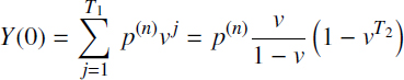
Let the net-premiums of value p(n) be paid in time 1, 2, …, T2 from the time of contract opening t0 = 0 to the time T2 = min{T1, T}. In this case, the premium can be considered as a life annuity of size p(n), which is paid to the insurer. Therefore, the reduced to the contract opening time t0 = 0 actuarial cost of the premium flow is equal to
Analogous values can be calculated for the time T of the contract completion.
3.4.4. The net-premium calculation
For the net-premium calculation, we focus on the case of both periodical payments (premiums and benefits) with equal values, as considered above. For the long-time as well as for the short-time insurance models, the premium calculation is based on the equity payments principle. To apply this principle, we should calculate the expectations of the benefit and premium PV, given by the formulas [3.32], [3.33]. It is convenient to represent the expectation of this value
which is called the actuarial present value of the contract cost, in the form E[X(0)] = bCb, where the value Cb is known as a benefit delayed annuity factor and calculated as
Analogously to the present value to the contract opening time t0 = 0, the actuarial cost of the premium flow that equals to the expectation of this sum is
and appropriate actuarial cost of the premium factor, which is the actuarial cost of the premium of an unit size flow Cp is calculated according to the formula
where ![]() is the m.g.f. of r.v. T2 in the point v.
is the m.g.f. of r.v. T2 in the point v.
Based on the equity payment principle, we should compare the expressions [3.34] and [3.35] and write
for any b. From this equation, the net-premium p(n) can be evaluated in the form
3.4.5. Insurance load calculation
In addition to the short-time insurance models, for a long-time insurance model, the net-premium provides equivalence between premiums and benefits only in mean. However, the insurer has to offset the expenses of its operation and provide the reliability of its own functioning. We will not focus here on the company operating expenses because it is only an economical question, and consider the problem of the reliability of company functioning. As with the short-time insurance models, the reliability of the company functioning means providing a negligibly small ruin probability.
In order to provide the given level of ruin probability, the premium also comprises the so-called insurance load p(s). Thus, in general, the premium p is calculated as a sum of net-premium p(n) and insurance load p(s), which is usually calculated in the fraction of the net-premium,
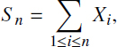
where Θ is the insurance load factor. So, let the company portfolio contain a sufficient number n of homogeneous contracts, of which the benefit of each is a r.v. ![]() . Thus, the summary benefit equals to
. Thus, the summary benefit equals to
which is supposed to be covered with the summary net-premium. The insurance load p(s) calculation, analogously to the case of short-time insurance models, is based on the principle of negligibly small ruin probability ψ of the company,
Under the assumption of independence of damages Xi for different contracts with expectation E[Xi] = μX and variance ![]() for the ruin probability calculation, we can use a normal approximation of the summary claim. Taking into account that the net-premium is calculated based on the payment equivalence principle, and in mean compensate the insurer’s expenses for the benefit payments, E[Sn] = np(n), for the ruin probability ψ using CLT, we can find
for the ruin probability calculation, we can use a normal approximation of the summary claim. Taking into account that the net-premium is calculated based on the payment equivalence principle, and in mean compensate the insurer’s expenses for the benefit payments, E[Sn] = np(n), for the ruin probability ψ using CLT, we can find

For a given ε appropriate quantile of the normal distribution z1-ε, such that the inequality fulfills

we can get the evaluation for insurance load in the form

Representing the insurance load as a fraction of net-premium, p(s) = Θ p(n), for the insurance load factor, we can find the following expression:
or in terms of variation coefficient ![]() in the form
in the form

Using, as before, the rough estimation of this value 3σ rule, according to which the probability of deviation of the normally distributed r.v. from its mean value that is more than three standard deviations is not greater than 0.1%, we can get

Using the above formulas for net-premium and insurance loads, we can find the value of complete premium,

3.4.6. An example
Illustrate the above reasonings with an artificial model of oil well insurance against depletion, proposed in section 3.1.5 (example 3.4). Suppose for the calculation that the distribution of time T1 is up to insurance event, when the oil well production rate (debit) becomes less, some critical values Q < Q* and the time T up to full termination of the well have discrete uniform distributions at the intervals [1, m] and [1, n] with m < n. It is an artificial assumption in order to propose some numerical results. In reality, these distributions need some special investigations.
In order to evaluate the present value of benefit PVX(0), we should remark that according to 3.32 for T1 < T,
Thus,

where qij is the joint distribution of r.v.’s T1 and T, under which condition, their independence is
Thus, we simply find that
and with simple algebra,
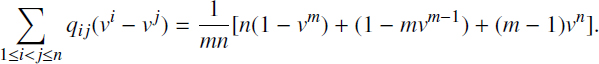
Finally, for E[PVX(0)], we have
Considering the case of small values of i and therefore also v close to one put v = 1 – ε. Therefore, taking into account that n >> 1 and m >> 1, we can put nε ≈ λ1 and mε ≈ λ2. Under this argument, we can find
This shows that the PV per unit benefit coefficient Cb is approximately equal to
On the one hand, the calculation of the net-premium present value PVY(0) expectation as

where ![]() is the value of the m.g.f. of the r.v. T2 = min(T1, T) distribution in the point v. This r.v. has the distribution
is the value of the m.g.f. of the r.v. T2 = min(T1, T) distribution in the point v. This r.v. has the distribution

Using this distribution, it is possible to calculate its m.g.f. ![]() . The calculations are cumbersome; however, the final expression is
. The calculations are cumbersome; however, the final expression is
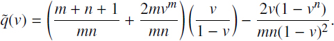
In this case of small interest rate i, when the discount factor v is close enough to one v = 1 – ε with the help of the m.g.f. Taylor expansion in the point v = 1, we can obtain

which show that the coefficient Cp is close to vE[T1].
Thus, for the value of premium evaluation, we have the following expression:
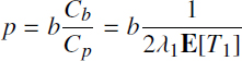
Evaluate the value of the premium for the case of annual payment of the benefit b = $100000 per year for interest rate i = 10%. It is possible to find that for the small value of interest rate i and therefore also the value of 1 – v, the value of the coefficient Cp is close to vE[T1], and for the value of coefficient Cb, we can find the approximation Cb ≈ (nϵ)-1. Thus, if the time of the well functioning with debit Q > Q* is uniformly distributed during 30 years, and the time to the well functioning up to the full closing is uniformly distributed during the 40 years, then
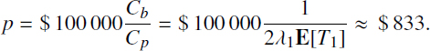
Therefore, in order to get the benefit of the value $100 000 each year during 10 years after the well loses the profit, it is enough to pay the premium of $ 833 per year during the previous 30 years.
3.4.7. Exercises
EXERCISE 3.21.– Calculate the insurance net-premium for an insurance contract with the mean benefit $ 10 000 in the case of an insurance event time occurrence that has an exponential distribution with the mean value λ-1 = 1, 000 days, under the condition of premium payment once a month with an interest rate of 10% per year.
3.5. Bibliographical comments
3.5.1. Section 3.1
Insurance practice and mathematics has a long history. First, the risk theory developed in the framework of actuarial mathematics has a ruin problem as a basic topic. New problems give a new push for its development. Usual terminology of insurance theory is used in this chapter (see [BOW 86]). Example 3.2 from section 3.1.5 about vehicle accidence insurance has been taken from [DAY 94]; example 3.4 from the same section has been considered in [RYK 98].
3.5.2. Section 3.2
The usual notions and methods of financial mathematics are used in this section [LYU 02, PAN 01, MAC 02].
3.5.3. Sections 3.3 and 3.4
In these sections the usual approaches for the investigation of short- and long-time insurance models are used.