
Chapter 4
Growth Curve Models
4.1 INTRODUCTION
In Chapters 2 and 3, we discussed the repeated measurements data analysis with univariate and multivariate methods. These methods are not always useful and have several restrictions imposed on them. To use the univariate methods, we require the dispersion matrix for the repeated measurements on units to satisfy the sphericity condition. This condition can be relaxed for multivariate methods. However, the multivariate methods require equal number of repeated measurements on each unit and the same covariates at each measurement time. The relaxation of this requirement needs a more broad-based linear and nonlinear models, and we will consider some such cases in this chapter.
In a dose–response curve, the responses are plotted against different dose levels (or log dose levels) of the drug. The response curve will be steep in a small window of required dose level and is nearly flat outside that window. Because of the slope pattern, these are known as sigmoidal (or S-shaped) curves. Some commonly used curves are based on logit, probit, and Gompertz models, and we will discuss them in Section 4.2.
A simple growth curve model can be used accounting for time-invariant and time-dependent covariates. We will consider them in Section 4.4 as linear models and in Section 4.5 as nonlinear models. Numerical examples are provided in Section 4.6. We will briefly discuss the mixed model analysis in Section 4.3 and the joint action models in Section 4.7.
4.2 Sigmoidal Curves
In some settings, the response variable Y is almost flat at the lower and higher values of the independent variable x and is steep in the effective domain of x. Such curves are known as sigmoidal curves and the underlying model is nonlinear. Some applications of such curves can be found in pharmacokinetics (Krug and Liebig, 1988; Liebig, 1988), toxicology (Becka and Urfer, 1996; Becka, Bolt, and Urfer, 1993), and other disciplines. Usually, x will be the dose (or log of the dose) level and Y will be the response for a drug.
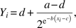
The general form of the nonlinear model can be written as
where Yi is the ith response, θ is the parameter vector of dimensionality p, xi is the ith dose or log of the ith dose (di), and ei are random errors. A suitable assumption of the errors can be made depending on the nature of the dose–response curve. While there is vast literature on finding the optimal choice of xi for a linear model (cf. Bose and Dey, 2009; Goos, 2002; Kiefer, 1958; Kunert, 1983; Pukelsheim, 1993; Shah and Sinha, 1989), limited work has been done on nonlinear models. The optimal designs for nonlinear models are given for minimal designs, where n = p; and the interested reader is referred to Antonello and Raghavarao (2000), Biedermann, Dette, and Zhu (2006), Chaudhuri and Mykland (1995), Dette, Melas, and Pepelyshev (2004), Kalish (1990), Dette, Melas, and Wong (2005), and Sitter and Torsney (1995) for details.
In Equation (4.2.1), θ will be estimated iteratively. We start with a vector of initial values, θ(0), and write
where

and where θ(a + 1) is substituted for θ in Equation (4.2.3).
Taking V to be the dispersion matrix of the error vector e′ = (e1, e2, …, en), by weighted least squares, we get
where

and
![]() θ(a + 1) - θ(a)
θ(a + 1) - θ(a)![]() ′
′![]() θ(a + 1) - θ(a)
θ(a + 1) - θ(a)![]() is less than a small predetermined bound δ.
is less than a small predetermined bound δ.
Note that H(a) is like the design matrix X in linear models. The estimated dispersion matrix of ![]() is
is
In general, we have four-parameter sigmoidal curves, where the parameters are denoted by a, b, c, and d.
We take the following:
- The plot Y versus x as sigmoid.
- When x = c, Y = (a + d)/2.
- Y is a function of x through b(x – c).
- When b > 0 (or <0), Y → d (or a) as x → –∞, and Y → a (or d) as x→∞.
Here, a and d are the extreme values of the response, b is the slope of the curve, and c is referred to as log(ED50) corresponding to a response proportion of 0.5.
The four-parameter family reduces to a three-parameter family by taking d to be known, say 0. It belongs to a two-parameter family by considering a and d to be known, say d = 0 and a = 1.
For simplicity, we denote b(xi – c) as ti and (Yi – d)/(a – d) as Pi and express the relationship between Y and x as
The model (4.2.1) becomes
The ith row of H(a), that is, X, can be written with four columns
where gi = g(ti) = (∂G(ti))/∂ti and Gi = G(ti).
With this X matrix and a suitable choice of V, we can determine the optimum Pi values, and they in turn based on historic data determine the optimum dose levels.
Logistic model is widely used and is given by

or equivalently
Probit and Gompertz models are also used in this context and are given by
and
respectively, where Φ(•) is the standard normal cumulative distribution function.
The ![]() estimator and its dispersion matrix can be obtained from SAS for different sigmoid curves. As an illustration, let us consider the effect of exercise time on weight loss. We will take eight volunteers with similar demographic variables and body weight. Artificial data of the exercise time in min (x, variable) and weight loss in lbs (Y, variable) after 3 months are given in Table 4.2.1.
estimator and its dispersion matrix can be obtained from SAS for different sigmoid curves. As an illustration, let us consider the effect of exercise time on weight loss. We will take eight volunteers with similar demographic variables and body weight. Artificial data of the exercise time in min (x, variable) and weight loss in lbs (Y, variable) after 3 months are given in Table 4.2.1.
Table 4.2.1 Artificial data of exercise time (X) and weight loss (Y)
| Volunteer | 1 | 2 | 3 | 4 | 5 | 6 | 7 | 8 |
| Exercise time (min) | 20 | 20 | 30 | 30 | 45 | 45 | 60 | 60 |
| Weight loss (lbs) | 4 | 5 | 15 | 16 | 30 | 32 | 35 | 38 |
The following programming lines provide the necessary output to draw inferences on the parameters:
data a; input x y@@; cards;
20 4 20 5 30 15 30 16 45 30 45 32 60 35 60 38
;
data b;set a;
proc nlin method = gauss ;
parms a = 50 b = .5 c = 30 d = 0;
model y = d + (a − d)/(1 + exp(−b * (x − c)));* this model fits the equation (4.2.10); run;
***| The NLIN Procedure | |||||||
| Approx | |||||||
| Parameter | Estimate | Std Error | Approximate 95% Confidence Limits | ||||
| (a1) | (a2) | (a3) | (a4) | ||||
| a | 37.8999 | 1.8455 | 32.7760 | 43.0238 | |||
| b | 0.1158 | 0.0298 | 0.0329 | 0.198 | |||
| c | 30.6832 | 2.8516 | 22.7660 | 38.6004 | |||
| d | −5.1965 | 6.7907 | −24.0506 | 13.6577 | |||
***

data a;
input x y@@;cards;
20 4 20 5 30 15 30 16 45 30 45 32 60 35 60 38
;
data b;set a;
proc nlin method = gauss ;
parms a = 50 b = .5 c = 30 d = 0;
model y = d + (a − d)* probnorm (b* (x − c));*this model fits equation (4.2.11); run;
***
| The NLIN Procedure | |||||||
| Approx | |||||||
| Parameter | Estimate | Std Error | Approximate 95% Confidence Limits | ||||
| (a5) | (a6) | (a7) | (a8) | ||||
| a | 37.1825 | 1.4965 | 33.0275 | 41.3376 | |||
| b | 0.0727 | 0.0184 | 0.0216 | 0.1237 | |||
| c | 30.5795 | 3.3837 | 21.1849 | 39.9742 | |||
| d | −4.7732 | 7.5297 | −25.6787 | 16.1323 | |||
***

data a;
input x y@@;cards;
20 4 20 5 30 15 30 16 45 30 45 32 60 35 60 38
;
data b;set a;
proc nlin method = gauss ;
parms a = 50 b = .5 c = 30 d = 0;
model y = d + (a − d)/(2** exp(−b * (x − c)));*this model fits equation (4.2.12);run;
***| The NLIN Procedure | |||||||
| Approx | |||||||
| Parameter | Estimate | Std Error | Approximate 95% Confidence Limits | ||||
| (a9) | (a10) | (a11) | (a12) | ||||
| a | 38.3101 | 2.0392 | 32.6483 | 43.9718 | |||
| b | 0.0987 | 0.0236 | 0.0332 | 0.1642 | |||
| c | 33.5640 | 1.4577 | 29.5168 | 37.6112 | |||
| d | 1.9127 | 3.2882 | −7.2169 | 11.0422 | |||
***
Using the column (a1), the fitted logistic model given in Equation (4.2.10) is
The standard errors of these parameters are given in column (a2) and the confidence intervals in [(a3), (a4)].
Using the column (a5), the fitted probit model given in Equation (4.2.11) is
The standard errors of these parameters are given in column (a6) and the confidence intervals in [(a7), (a8)].
Using the column (a9), the fitted Gompertz model given in Equation (4.2.12) is

The standard errors of these parameters are given in column (a10) and the confidence intervals in [(a11), (a12)].
The estimated parameters of a, b, c, and d for the three models are summarized in Table 4.2.2. From this table, we observe that parameter estimates of a, b, and c are reasonably close for these models, whereas d is slightly higher for Gompertz model.
Table 4.2.2 Comparison of the parameter for the three models
| Parameter | Logistic | Probit | Gompertz |
| a | 37.8999 | 37.1825 | 38.3101 |
| b | 0.1158 | 0.0727 | 0.0987 |
| c | 30.6832 | 30.5795 | 33.5640 |
| d | −5.1965 | −4.7732 | 1.9127 |
The D-optimal designs are compromised of those design points that minimize the determinant of the variance–covariance matrix of the estimated parameters. Box (1971) showed that the D-optimality criterion is desirable because it tends to reduce the biases of the maximum likelihood estimates of the parameters in nonlinear models. We will now illustrate the method of determining D-optimum minimal design pi’s for a two-parametric logistic model with a = 1 and d = 0.
Here, the model is
and the H-matrix (or equivalently the design matrix X) is

Let us assume binomial variation of errors and take
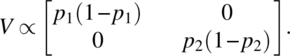
Maximizing |X′V− 1X| is equivalent to maximizing |X′V− 1/2|. We now have

Differentiating |X′V− 1/2| with respect to p1 and p2 and equating to zero, we get
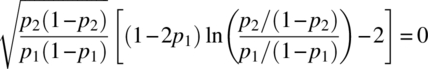
and

Solving for p1 and p2 from the two Equations (4.2.14) and (4.2.15), we get
The dose levels corresponding to these response proportions are the optimum design points. This result was obtained by Kalish and Rosenberger (1978) and also by Antonello and Raghavarao (2000). By using similar methods, we can determine optimal pi values for minimal designs.
Testing the lack of fit of minimal designs is very important for these models, and the interested reader is referred to Lupinacci and Raghavarao (2000) and Su and Raghavarao (2013).
4.3 Analysis of Mixed Models
The analysis of growth curves requires some understanding of restricted maximum likelihood (REML) and penalized least squares, and in this section, a brief summary of these methods will be provided.
Consider a mixed model
where Y is a n × 1 random vector of responses, β is a r × 1 vector of fixed effect parameters and u is a p × 1 vector of random effect parameters, e is random error, and X and Z are design matrices of fixed and random effects. For simplicity, we assume X to be of rank r, and this can always be accomplished by reparametrizing the parameters of the vector β. We assume u to have a multivariate normal distribution Np(0, G) and e to have a multivariate normal distribution Nn(0, R); u and e are independent. Usually, G and R will be diagonal matrices. We assume G and R to be nonsingular. We have
The best linear unbiased estimator ![]() of β and the best linear unbiased predictor
of β and the best linear unbiased predictor ![]() of u can be obtained by minimizing
of u can be obtained by minimizing
with respect to β and u. This process is known as penalized least squares. The resulting normal equations by minimizing the penalized least squares (Eq. 4.3.4) are
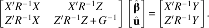
Note that

From the second Equation of (4.3.5), we have
and substituting this in the first Equation of (4.3.5), we get
which simplifies to
The estimated ![]() of Equation (4.3.8) can also be obtained as weighted least squares estimator for the model
of Equation (4.3.8) can also be obtained as weighted least squares estimator for the model
We can also verify
so that Equation (4.3.7) gives
If V is known, we can solve for ![]() from Equation (4.3.8). If V is unknown, we need to estimate it and we will do this by REML.
from Equation (4.3.8). If V is unknown, we need to estimate it and we will do this by REML.
Let K be a n × (n–r) matrix such that
and make the transformation
so that
We observe

and
Since the determinants of the left-hand side Equations of (4.3.15) and (4.3.16) are the same, we have
Put M = I − X(X′V−1 X)−1X′V−1, and note
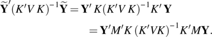
Clearly, V is a g-inverse of K(K′VK)− 1K′, as
Let
so that
and
Substituting Equations (4.3.19) and (4.3.20) in Equation (4.3.18),
The log likelihood of V, using the distribution of Y and ignoring the constant expression, is

By differentiating ![]() with respect to the parameters of G and R and solving the equations, we estimate V and subsequently β. In SAS, procedure PROC MIXED provides the necessary output to draw inferences on the parameters, and we will illustrate this in the following example:
with respect to the parameters of G and R and solving the equations, we estimate V and subsequently β. In SAS, procedure PROC MIXED provides the necessary output to draw inferences on the parameters, and we will illustrate this in the following example:
Table 4.3.1 Average class GPA based on teaching method and instructor
| Teacher | A | B | C | A | B | C | A | B | C |
| Method | 1 | 2 | 3 | 2 | 3 | 1 | 3 | 1 | 2 |
| Class GPA | 2.9 | 3.1 | 2.9 | 3.0 | 3.4 | 2.8 | 3.0 | 2.6 | 2.8 |
We assume the model
where Yij is the class GPA, with jth teacher and ith teaching method; βi is the fixed effect of ith method; uj is the random effect of jth teacher; uij is the random interaction effect of the ith method and jth instructor; and eij are random errors. All the random effects parameters are assumed to have zero mean. The parameters uj, uij, and eij are assumed to have variances ![]() ,
, ![]() , and σ2, respectively. Further, uj and eij are assumed to be independent, as well as uij and eij. The parameters uj and uij are assumed to have σ12 covariance.
, and σ2, respectively. Further, uj and eij are assumed to be independent, as well as uij and eij. The parameters uj and uij are assumed to have σ12 covariance.
The necessary programming lines and output are given as follows:
data a;
input teacher method gpa @@;cards;
1 1 2.9 2 2 3.1 3 3 2.9 1 2 3.0 2 3 3.4 3 1 2.8 1 3 3.0 2 1 2.6 3 2 2.8
;
data c;set a;
proc mixed covtest;
class teacher ;*In this program we are not considering method as a class variable;
model gpa = method /s;
random int method /type = un sub = teacher cl; run;

***
| Iteration History | |||
| Iteration | Evaluations | −2 Res Log Like | Criterion |
| 0 | 1 | 0.11209305 | |
| 1 | 1 | −6.90241885 | 0.00000000 |
| Convergence criteria met. | |||
| The Mixed Procedure | |||||
| Covariance Parameter Estimates | |||||
| Standard | Z | ||||
| Cov Parm | Subject | Estimate | Error | Value | Pr Z |
| (b1) | (b2) | ||||
| UN(1,1) | teacher | 0.1037 | 0.1117 | 0.93 | 0.1765 (b3) |
| UN(2,1) | teacher | −0.06278 | 0.06685 | −0.94 | 0.3477 (b4) |
| UN(2,2) | teacher | 0.03917 | 0.04086 | 0.96 | 0.1689 (b5) |
| Residual | 0.003333 | 0.002722 | 1.22 | 0.1103 | |
| Fit Statistics | |
| −2 Res Log Likelihood | −6.9 |
| AIC (smaller is better) | 1.1 |
| AICC (smaller is better) | 21.1 |
| BIC (smaller is better) | −2.5 |
| Null Model Likelihood Ratio Test | ||
| DF | Chi-Square | Pr > ChiSq |
| 3 | 7.01 | 0.0714 |
| Solution for Fixed Effects | |||||
| Standard | |||||
| Effect | Estimate | Error | DF | t Value | Pr > |t| |
| Intercept | 2.6111 | 0.1928 | 2 | 13.55 | 0.0054 |
| method | 0.1667 | 0.1167 | 2 | 1.43 | 0.2893 |
| Solution for Random Effects | |||||||||||||||
| Std Err | |||||||||||||||
| Effect | teacher | Estimate | Pred | DF | t Value | Pr > |t| | Alpha | Lower | Upper | ||||||
| (b7) | |||||||||||||||
| Intercept | 1 | 0.2103 | 0.1968 | 3 | 1.07 | 0.3635 | 0.05 | −0.4159 | 0.8366 | ||||||
| method | 1 | −0.1024 | 0.1186 | 3 | −0.86 | 0.4514 | 0.05 | −0.4798 | 0.2750 | ||||||
| Intercept | 2 | −0.3587 | 0.1968 | 3 | −1.82 | 0.1658 | 0.05 | −0.9850 | 0.2675 | ||||||
| method | 2 | 0.2238 | 0.1186 | 3 | 1.89 | 0.1555 | 0.05 | −0.1536 | 0.6012 | ||||||
| Intercept | 3 | 0.1484 | 0.1968 | 3 | 0.75 | 0.5055 | 0.05 | −0.4778 | 0.7746 | ||||||
| method | 3 | −0.1214 | 0.1186 | 3 | −1.02 | 0.3812 | 0.05 | −0.4988 | 0.2559 | ||||||
| The Mixed Procedure | ||||
| Type 3 Tests of Fixed Effects | ||||
| Num | Den | |||
| Effect | DF | DF | F Value | Pr > F |
| method | 1 | 2 | 2.04 | 0.2893 (b6) |
From the output in column (b1), we get the estimators for ![]() , σ12,
, σ12, ![]() , and σ2 and its standard error in column (b2). The p-values at (b3), (b4), and (b5) can be used to test the significance of
, and σ2 and its standard error in column (b2). The p-values at (b3), (b4), and (b5) can be used to test the significance of ![]() , σ12, and
, σ12, and ![]() . The p-value at (b6) is used to test the significance of the fixed effect parameter, and in our case, it is not significant. The p-values in column (b7) can be used to test the significance of intercepts and slope for the methods with each teacher.
. The p-value at (b6) is used to test the significance of the fixed effect parameter, and in our case, it is not significant. The p-values in column (b7) can be used to test the significance of intercepts and slope for the methods with each teacher.
For more details, the interested readers are referred to Harville (1977), Searle, Casella, and McCulloch (1992), and Patterson and Thompson (1971).
4.4 Simple Linear Growth Curve Model
Let us consider n experimental units and the maximum number of repeated measures on any unit is T. However, it is not necessary to have all T observations on every unit. Let ti(≤T) be the number of repeated observations on the ith unit. Let aij denote a time score for the jth observation on the ith unit. Let X1, X2, …, XM be the M time-invariant covariates and let W1, W2, …, WL be the L time-variant covariates. We will assume a two-stage linear model. Let Yij be the response on the jth observation on the ith unit. We assume

where ![]() is value of the
is value of the ![]() covariate
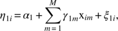
covariate ![]() at the jth observation on the ith unit and we take it to be zero, if no data are available; eij are random errors; η0i is intercept; and η1i and
at the jth observation on the ith unit and we take it to be zero, if no data are available; eij are random errors; η0i is intercept; and η1i and ![]() are slopes. We model the parameters as follows using the time-invariant covariates:
are slopes. We model the parameters as follows using the time-invariant covariates:


where ξ0i, ξ1i, and ![]() are random errors and γ’s are slopes of the time-invariant covariates. We will take xim to be zero if the data on Xi are not available.
are random errors and γ’s are slopes of the time-invariant covariates. We will take xim to be zero if the data on Xi are not available.
Combining Equations (4.4.1)–(4.4.4), we write the response vector Yi′ of dimension ti as
where 1 is a column vector of 1’s of suitable dimension (i.e., Jt,1), ![]() ,
, ![]() ,
, ![]() ,
, ![]() ,
, ![]() is a tj × L matrix,
is a tj × L matrix, ![]() ,
, ![]() is a L × M matrix,
is a L × M matrix, ![]() , and
, and ![]() . In xi, and Wi, we put 0 values when data are not collected on those variables at the indicated response time.
. In xi, and Wi, we put 0 values when data are not collected on those variables at the indicated response time.
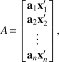
Let ![]() . We combine the expression of the response vectors of Equation (4.4.5) to get an N component vector response
. We combine the expression of the response vectors of Equation (4.4.5) to get an N component vector response ![]() as
as
In Equation (4.4.6), X is an N × M matrix
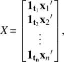
![]() ; A is an N × M matrix
; A is an N × M matrix
W is an N × L matrix


B is an N × L vector matrix

and ![]() .
.
Model (4.4.6) is a mixed effects model, where the last four terms give random effects parameter and the remaining terms are fixed effects parameter. The effect of the M time-invariant covariates X1, X2, …, XM can be tested by testing the parameters γ01, γ02, …, γ0M. The effect of the L time-variant covariates W1, W2, …, WL can be tested by testing the parameters α21, α22, …, α2L. The effects of the time scores can be tested by testing the parameters γ11, γ12, …, γ1M. The interaction between the set of parameters ![]() and {WM} can be tested by testing the parameters
and {WM} can be tested by testing the parameters ![]() for
for ![]() ; m = 1, 2, …, M.
; m = 1, 2, …, M.
4.5 Nonlinear Growth Curve Model
Continuing the notation of Section 4.4, for simplicity, we assume one time-variant covariate, W, and one time-invariant covariate, X. Let tij be the score indicating the repetition of the observation on the unit. We can assume any nonlinear model for repeated observations on a unit and also with a time-invariant covariate.
Let us assume the logistic model for repeated observations as

We model the coefficients ![]() for
for ![]() of Equation (4.5.1) as
of Equation (4.5.1) as
Substituting Equations (4.5.2)–(4.5.5) in Equation (4.5.1), we obtain

Usually, the covariate wij in Equation (4.5.1) is considered with coefficient 1; however, for generality, we consider its coefficient bi1.
4.6 Numerical Example
In this section, the linear and nonlinear growth curves will be illustrated. Example 4.6.1 illustrates fitting the linear growth curve model, and Example 4.6.2 illustrates fitting the nonlinear model.
Table 4.6.1 Artificial data on change of A1C
| Patient | 3 m | 6 m | 9 m | |||||
| X i1 | X i2 | W ij1 | yij | W ij1 | yij | W ij1 | yij | |
| 1 | 170 | 60 | 20 | +0.2 | 30 | −0.5 | 30 | +0.1 |
| 2 | 220 | 55 | 40 | −0.1 | 35 | −0.6 | 30 | −0.1 |
| 3 | 180 | 40 | 50 | −0.5 | 40 | 0.1 | 45 | −0.2 |
| 4 | 200 | 50 | 30 | −0.1 | 40 | −0.1 | 40 | +0.1 |
| 5 | 185 | 60 | 10 | −0.3 | 30 | −0.1 | 30 | −0.1 |
data a;
input patient period xi1 xi2 aj wi1 y@@;cards;
1 1 170 60 3 20 .2 1 2 170 60 6 30 -.5 1 3 170 60 9 30 .12 1 220 55 3 40 -.1 2 2 220 55 6 35 -.6 2 3 220 55 9 30 -.13 1 180 40 3 50 -.5 3 2 180 40 6 40 .1 3 3 180 40 9 45 -.24 1 200 50 3 30 -.1 4 2 200 50 6 40 -.1 4 3 200 50 9 40 .15 1 185 60 3 10 -.3 5 2 185 60 6 30 -.1 5 3 185 60 9 30 -.1
;

data b;set a;
%macro est(in,patno);
data c;set a;
if patient = &patno; proc sort; by patient;

ods trace on;
proc glm outstat = z ;
model y = aj wi1 /noint ;
*no intercept is used because not enough period observations are taken;
ods output parameterestimates = all; output out = aa; run;

data all1; set all; keep estimate parameter ;
proc transpose out = allt; var estimate parameter;
data allt; set allt; patient = &patno; if _name_ = 'Estimate';
ajhat = col1 + 0; wi1hat = col2 + 0; drop col1 col2;
patient = &patno; proc sort; by patient; drop col1 col2 col3;

data all2; set all; keep stderr parameter ;
proc transpose out = allt2; var stderr parameter;
data allt2; set allt2; patient = &patno; if _name_ = 'StdErr';
seajhat = col1 + 0; sewi1hat = col2 + 0; drop col1 col2;
patient = &patno; proc sort; by patient; drop col1 col2 col3;

data all3; set all; keep probt parameter ;
proc transpose out = allt3; var probt parameter;
data allt3; set allt3; patient = &patno; if _name_ = 'Probt';
ajpvalue = col1 + 0; wi1pvalue = col2 + 0; drop col1 col2;
patient = &patno; proc sort; by patient; drop col1 col2 col3;

data z1;set z; if _source_ = 'ERROR';
patient = &patno; keep ss patient; proc sort; by patient;

data zz;merge allt c z1 allt2 allt3;by patient;

data ∈set zz;
keep ajhat seajhat wi1hat sewi1hat xi1 xi2 ss ajpvalue wi1pvalue;
if _n_ = 1;
%mend est;
%est(pat1,1);%est(pat2,2);%est(pat3,3);%est(pat4,4);%est(pat5,5);

data final;set pat1 pat2 pat3 pat4 pat5;
errorMS = SS; drop ss probt;

data final2;set final;
proc print; var ajhat seajhat ajpvalue wi1hat sewi1hat wi1pvalue errorms;run;

Output (c1) :
| Obs | ajhat | seajhat | ajpvalue | wi1hat | sewi1hat | wi1pvalue | errorMS |
| 1 | 0.045614 | 0.18103 | 0.8429 | −0.014211 | 0.043324 | 0.7982 | 0.25474 |
| 2 | −0.009877 | 0.07535 | 0.9170 | −0.005926 | 0.013858 | 0.7428 | 0.16667 |
| 3 | 0.052335 | 0.06301 | 0.5588 | −0.011691 | 0.009038 | 0.4190 | 0.09058 |
| 4 | 0.051111 | 0.01423 | 0.1729 | −0.009333 | 0.002494 | 0.1663 | 0.00200 |
| 5 | −0.026667 | 0.11624 | 0.8564 | 0.002000 | 0.029933 | 0.9575 | 0.06400 |
data final1; set final;
proc glm; model ajhat = xi1 xi2; run;
proc glm; model wi1hat = xi1 xi2; run;
| The GLM Procedure | |||||
| Dependent Variable: ajhat | |||||
| Source | DF | Sum of Squares | Mean Square | F Value | Pr > F |
| Model | 2 | 0.00286544 | 0.00143272 | 1.01 | 0.4980 |
| Error | 2 | 0.00284314 | 0.00142157 (c2) | ||
| Corrected Total | 4 | 0.00570858 | |||
***
| Parameter | Estimate | Standard Error | t Value | Pr > |t| |
| (c3) | (c4) | (c5) | ||
| Intercept | 0.3169810450 | 0.22294561 | 1.42 | 0.2910 |
| xi1 | −.0008153084 | 0.00096733 | −0.84 | 0.4880 |
| xi2 | −.0026179955 | 0.00225382 | −1.16 | 0.3653 |
| The GLM Procedure | |||||
| Dependent Variable: wi1hat | |||||
| Source | DF | Sum of Squares | Mean Square | F Value | Pr > F |
| Model | 2 | 0.00004202 | 0.00002101 | 0.36 | 0.7343 |
| Error | 2 | 0.00011611 | 0.00005806 (c6) | ||
| Corrected Total | 4 | 0.00015813 | |||
***
| Parameter | Estimate | Standard Error | t Value | Pr > |t| |
| (c7) | (c8) | (c9) | ||
| Intercept | −.0443513365 | 0.04505511 | −0.98 | 0.4287 |
| xi1 | 0.0001076860 | 0.00019549 | 0.55 | 0.6370 |
| xi2 | 0.0003009658 | 0.00045548 | 0.66 | 0.5767 |
In Part (c1) of the output, the individual patients analysis are given. One can determine the significance of the parameters from that output. In (c2) and (c6), the error mean squares are provided for the parameters aj’s and wi1. The estimates, standard errors, and p-values are given for the second-stage parameters in columns (c3)–(c5) and (c7)–(c9).
Table 4.6.2 Artificial data on weight loss
| Volunteer | Xi | Wij, tij, yij |
| 1 | 1200 | (20, 3, 3) (40, 6, 5) (25, 9, 3.5) (30, 12, 4) |
| 2 | 1200 | (20, 3, 4) (25, 6, 5) (60, 12, 9) (40, 9, 7) |
| 3 | 1200 | (25, 6, 5) (40, 9, 7) (60, 12, 9) (30, 3, 5) |
| 4 | 1500 | (20, 3, 4) (25, 6, 5) (40, 9, 7) (60, 12, 10) |
| 5 | 1500 | (25, 6, 5) (40, 9, 6) |
| 6 | 1500 | (25, 6, 4) (40, 9, 6) (60, 12, 8) |
The following programming lines provide the necessary output to draw inferences:
data a;input patient x w t y @@;cards;
1 1200 20 3 3 1 1200 40 6 5 1 1200 25 9 3.5 1 1200 30 12 4
2 1200 20 3 4 2 1200 25 6 5 2 1200 60 12 9 2 1200 40 9 7
3 1200 25 6 5 3 1200 40 9 7 3 1200 60 12 9 3 1200 30 3 5
4 1500 20 3 4 4 1500 25 6 5 4 1500 40 9 7 4 1500 60 12 10
5 1500 25 6 5 5 1500 40 9 6
6 1500 25 6 4 6 1500 40 9 6 6 1500 60 12 8
;
proc sort;by patient;

Step 1: Summarize the parameters b1, b2, b3 and b4 for the 6 patients

data b;set a;
%macro est(subject,out);

data c;  set b;
if patient = &subject;
proc nlin noprint;   parms b1 = .1 b2 = 3 b3 = .5 b4 = 1;
model y = ((b1*w) + b4)/(1 + exp(−(t−b2)/b3)); output out = &out parms = b1 b2 b3 b4; run;
data &out ;set &out;
proc sort nodupkey;by patient;
%mend est;

%est(1,out1); %est (2,out2); %est (3,out3);
%est(4,out4); %est (5,out5); %est (6,out6);

data final;set out1 out2 out3 out4 out5 out6;
data final1; set final;  keep patient b1 b2 b3 b4;  proc print; run;
| (d1) | |||||
| Obs | patient | b1 | b2 | b3 | b4 |
| 1 | 1 | 0.10000 | −6.1601 | 0.61366 | 1.00000 |
| 2 | 2 | 0.07514 | −8.7579 | 4.17192 | 3.20507 |
| 3 | 3 | 0.07329 | −9.2748 | 3.44509 | 3.68037 |
| 4 | 4 | 0.14324 | 2.7534 | 0.08630 | 1.36486 |
| 5 | 5 | 0.12492 | −48.3823 | 0.50000 | 1.00000 |
| 6 | 6 | 0.09991 | 4.9635 | 0.50000 | 2.00560 |
Step 2: We will take b1, b2, b3 and b4 given at (d1) of the output and regress these values using the X values of the dependent variable.
data final1;set final;
proc glm; model b1 = x; run;

***
| Parameter | Estimate | Standard Error | t Value | Pr > |t| |
| (d2) | (d3) | (d4) | ||
| Intercept | −.0575655521 | 0.06562982 | −0.88 | 0.4299 |
| x | 0.0001201708 | 0.00004832 | 2.49 | 0.0677 |
 proc glm;  model b2 = x;  run;
***
| Parameter | Estimate | Standard Error | t Value | Pr > |t| |
| (d5) | (d6) | (d7) | ||
| Intercept | 4.634195173 | 79.74988058 | 0.06 | 0.9564 |
| x | −0.012126211 | 0.05871267 | −0.21 | 0.8465 |
proc glm;  model b3 = x;  run;
***
| Parameter | Estimate | Standard Error | t Value | Pr > |t| |
| (d8) | (d9) | (d10) | ||
| Intercept | 11.89518939 | 4.85592335 | 2.45 | 0.0705 |
| x | −0.00768873 | 0.00357498 | −2.15 | 0.0979 |
proc glm;  model b4 = x;  run;
***
| Parameter | Estimate | Standard Error | t Value | Pr > |t| |
| (d11) | (d12) | (d13) | ||
| Intercept | 6.298067264 | 3.49427421 | 1.80 | 0.1458 |
| x | −0.003227497 | 0.00257252 | −1.25 | 0.2779 |
The parameters b1, b2, b3, and b4 for individual patients are summarized at (d1) of the output. The individual linear regressed parameters β1, β2, β3, and β4 are given in the columns (d2), (d5), (d8), and (d11) of the output. The standard errors of these parameters are given in columns (d3), (d6), (d9), and (d12). The p-values for testing these parameters are given in the columns (d4), (d7), (d10), and (d13). In our example, none of these parameters are significant.
In Table 4.6.2, artificial data with different periods was given on the volunteers to show that we can use this kind of general modeling when all periods data are not available on the subjects.
4.7 Joint Action Models
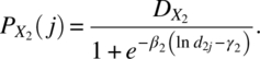
In Section 4.2, we discussed some sigmoidal curves for single-compound dose–response models. The general logistic regression model with one compound X can be rewritten as
Here,
where β indicates the steepness of the dose–response function; γ is ln(dose) corresponding to a response proportion of 0.5, or ln(ED50); di is the ith dose level; and Dx is an indicator variable taking the value 1 (or 0) according to di > 0 (or di = 0), ymin and ymax being the minimum and maximum responses.
Joint action refers to the response of an individual to a combination of compounds. The combination of two compounds X1 and X2 can produce an “additive” or a “nonadditive” response. When the response is additive, no interaction exists between the two compounds. When the response is nonadditive, an interaction exists between the two compounds.
Synergism and antagonism are two terms used to describe the nonadditive joint action. Synergism is when the two compounds work together to produce an effect greater than that which would be expected by the two compounds working alone. Antagonism is when the two compounds work in competition with one another to produce an effect that is less than that which would be expected by the two compounds working alone (Ashford, 1981; Lupinacci, 2000).
From the selection of the appropriate additive and nonadditive joint action model come the concepts of “similar joint action” and “independent joint action.” Compounds competing against one another to work in the same area of the body and in the same manner are known as similar joint action. Compounds working in different areas of the body and by different methods of action are known as independent joint action (Ashford, 1981; Lupinacci, 2000).
In this monograph, we will restrict ourselves to the additive and nonadditive independent joint action models.
Let X1 and X2 be two compounds administered at d1i and d2j levels, then the additive joint response under independent joint action, Yij, can be written (see Barton, Braunberg, and Friedman, 1993) as
where ymin and ymax are defined as earlier and
The data can be analyzed under different assumptions on the error. By writing the model in a linear form using Taylor’s expansion, Antonello and Raghavarao (2000) gave the optimum dose levels.
In the case of nonadditivity, Barton, Braunberg, and Friedman (1993) considered the model
where
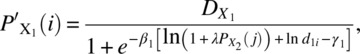
and

The optimal design points in the nonadditive case are also given by Antonello and Raghavarao (2000). In Equations (4.7.7) and (4.7.8), λ is known as nonadditivity parameter. Clearly, λ = 0 for additive joint action.
Table 4.7.1 Artificial data on the percentage reduction of diastolic BP
| d i1 (mg) | d i2 (mg) | yij |
| 15 | 25 | 9 |
| 15 | 75 | 9 |
| 50 | 25 | 12 |
| 50 | 75 | 11 |
| 25 | 50 | 10 |
The following programming lines fit the additive independent joint action model (4.7.3) assuming ymin = 0, ymax = 15 to be known:
data a;
input d1 d2 y @@;cards;
15 25 9 15 75 9 50 25 12 50 75 11 25 50 10
;

proc nlin;
parms beta1 = 1 beta2 = 1.5 gamma1 = 5 gamma2 = 4;
model y = ( (1/(1 + exp(−beta1*(log(d1)−gamma1)))) +(1/(1 + exp(−beta2*(log(d2)−gamma2))))−(1/(1 + exp(−beta1*(log(d1)−gamma1))))*(1/(1 + exp(−beta2*(log(d2)−gamma2)))) )*15;  run;

***

NOTE: Convergence criterion met.

***
| The NLIN Procedure | |||||
| Source | DF | Sum of Squares | Mean Square | F Value | Approx Pr > F |
| Model | 4 | 526.6 | 131.7 | 353.38 | 0.0399 (e1) |
| Error | 1 | 0.3726 | 0.3726 | ||
| Uncorrected Total | 5 | 527.0 | |||
| Approx | |||||||
| Parameter | Estimate | Std Error | Approximate 95% Confidence Limits | ||||
| (e2) | (e3) | (e4) | |||||
| beta1 | 0.6573 | 0.1750 | −1.5668 | 2.8814 | |||
| beta2 | −2.9541 | 37.8159 | −483.4 | 477.5 | |||
| gamma1 | 2.1875 | 0.5865 | −5.2649 | 9.6399 | |||
| gamma2 | 2.3591 | 10.2145 | −127.4 | 132.1 | |||
***
From the output, the p-value given at (e1) tests for the significance of the model and our p-value is significant. The estimated model parameters β1, β2, γ1, and γ2 are given in column (e2). The lower and upper CI for these parameters are given in columns (e3) and (e4).
A similar program as can also be given for the model (4.7.6) in the case of nonadditive joint action model.
References
- Antonello JM, Raghavarao D. Optimal designs for the individual and joint exposure general logistic regression models. J Biopharm Statist 2000;10:351–367.
- Ashford JR. General models for the joint action of mixtures of drugs. Biometrics 1981;37:457–474.
- Barton CN, Braunberg RC, Friedman L. Nonlinear statistical models for the joint action of toxins. Biometrics 1993;49:95–105.
- Becka M, Urfer W. Statistical aspects of inhalation toxicokinetics. Environ Ecol Statist 1996;3:51–64.
- Becka M, Bolt HM, Urfer W. Statistical evaluation of toxicokinetic data. Environmetrics 1993;4:311–322.
- Biedermann S, Dette H, Zhu W. Optimal designs for dose–response models with restricted design spaces. J Am Statist Assoc 2006;101:747–759.
- Bose M, Dey A. Optimal Cross-Over Designs. Singapore: World Scientific; 2009.
- Box MJ. Bias in nonlinear estimation. J R Statist Soc B 1971;33:171–201.
- Chaudhuri P, Mykland PA. On efficient designing of nonlinear experiment. Statist Sin 1995;5:421–440.
- Dette H, Melas VB, Pepelyshev A. Optimal designs for a class of nonlinear regression models. Ann Math Statist 2004;32:2142–2167.
- Dette H, Melas VB, Wong WK. Optimal designs for goodness-of-fit of the Michaelis–Menton enzyme kinetic function. J Am Statist Assoc 2005;100:1370–1381.
- Goos P. The Optimal Design of Blocked and Split-Plot Experiments. New York: Springer-Verlag; 2002.
- Harville DA. Maximum likelihood approaches to variance component estimation and to related problems. J Am Statist Assoc 1977;72:320–338.
- Kalish LA. Efficient design for estimation of median lethal dose and quantal dose–response curves. Biometrics 1990;46:737–748.
- Kalish LA, Rosenberger JL. Optimal designs for the estimation of the logistic function. Technical Report 33. University Park, PA: Pennsylvania State University; 1978.
- Kiefer J. On the nonrandomized optimality and randomized nonoptimality of symmetric designs. Ann Math Statist 1958;29:675–699.
- Krug H, Liebig HP. Static regression models for planning greenhouse production. Acta Horticult 1988;230:427–433.
- Kunert J. Optimal design and refinement of the linear model with applications to repeated measurements designs. Ann Math Statist 1983;11:247–257.
- Liebig HP. Temperature integration by kohlrabi growth. Acta Horticult 1988;230:427–433.
- Lupinacci PJ. d-Optimal designs for a class of nonlinear models [unpublished Ph.D. dissertation]. Philadelphia, PA: Temple University; 2000.
- Lupinacci PJ, Raghavarao D. Designs for testing lack of fit for a nonlinear dose–response curve model. J Biopharm Statist 2000;10:45–53.
- Patterson HD, Thompson R. Recovery of inter-block information when block sizes are unequal. Biometrika 1971;58:545–554.
- Pukelsheim F. Optimal Design of Experiments. New York: Wiley; 1993.
- Searle SR, Casella G, McCulloch CE. Variance Components. New York: Wiley; 1992.
- Shah KR, Sinha BK. Theory of Optimal Designs. Lecture Notes in Statistic. New York: Springer; 1989.
- Sitter RR, Torsney B. Optimal designs for binary response experiments with two design variables. Statist Sin 1995;5:405–419.
- Su Y, Raghavarao D. Minimal plus one point designs to test lack of fit for some sigmoidal curves. J Biopharm Statist 2013;23:281–293.