
6 Introduction to Critical Path and Schedule Risk Analysis
Recognising the need to plan is the first step towards arriving at a successful outcome. The reverse is certainly true, as the popular unverified quotation states: if we don’t plan, we shouldn’t expect to be successful … but we might just get lucky! (Hmm, try telling your director that and see how long you get to stay in the same room!)
Every estimator should be able to plan in support of a robust Estimating Process (see Volume I Chapter 2). If they are cost estimators, they also need to be able to understand the implications of a plan or schedule in terms of the interaction between cost and schedule.
A word (or two) from the wise?
'Failing to plan is planning to fail.' Popular Quotation (Unverified) Attributed in various forms to:
Benjamin Franklin
US President
Winston Churchill
UK Prime Minister
and Alan Lakein
Time Management Consultant
If everything in life was sequential, the life of the planner, scheduler and estimator would be so much simpler, but everyone else would have to learn to be patient as many things would take a lot longer to achieve than they do now, when inevitably, some tasks are performed in parallel. So, how much work can be performed in parallel? This is where Critical Path Analysis can come to our aid.
6.1 What is Critical Path Analysis?
To speed things up, we can (and do) allow some tasks or activities to occur in parallel, but there is normally a physical limit or constraint in terms of a natural sequence of pre-requisite tasks or activities. For instance, we cannot derive the numerical value of an estimate in parallel to the agreement of the assumptions which underpin it; the latter is a pre-requisite of the former. The overall time from start to finish is determining by this natural sequence and the task/activity durations.
We can draw these tasks/activities and the inherent dependencies as a logic network diagram. A search of the internet will show us that there are many different styles in use. Some are better than others in conveying the essential information; the key thing is to choose a style that works best for us and our individual organisations. The styles really fall into two camps:
- Activity on Node: Each task or activity is drawn on node represented by a geometric shape (e.g. circle or rectangle). They are joined by lines indicating the direction of logical flow to our next task or activity and are labelled or annotated accordingly
- Activity on Arrow: Each task or activity begins and ends at a node. The nodes represent the logical points by which parallel tasks/activities must ‘come together’ or can divide. The arrows or boxes between the nodes represent the tasks/activities and are labelled or annotated accordingly
The essential information we must input to the network is:
- Any required preceding tasks or activities
- Any required succeeding tasks or activities
- Each task or activity’s expected duration
From the network, we can derive the earliest and latest start and finish times for each task or activity, and any slack or float time that can be used to vary start or finish times of individual tasks or activities, should the need arise. It also allows us to identify the Critical Path, i.e. that route through the network where no float is available if we want to achieve the earliest start to finish time for the project overall.
Definition 6.1 Critical Path
The Critical Path at a point in time depicts the string of dependent activities or tasks in a schedule for which there is no float or queuing time. As such the length of the Critical Path represents the quickest time that the schedule can be expected to be completed based on the current assumed activity durations and associated circumstances.
The question now arises on whether the earliest start time of the first activity is at time zero, or time 1 (or any other time for that matter). Furthermore, we might also ask ourselves whether we are assuming that each activity ends in the middle of the time period, or at the end, and whether the next activity starts immediately or in the next time period. For example, consider two activities with durations of four and five time periods; Table 6.1 summarises the two options available to us. It doesn’t matter which option we choose so long as we are consistent. We can always work with the simplest option first (Option 0, the null option) and convert to the other option later. We will be adopting Option 0 in the examples that follow.
Let’s look at an example. In Figure 6.1 we have shown the Network Diagram for a Plan to develop a Time-phased Estimate including an appropriate level of Risk and Uncertainty Contingency using an ‘Activity on Node’ format, and using the start/finish times at the mid-point of the time intervals (Option 0).
We will notice that there is a table of data underpinning each activity (we will get back to the calculations shortly … I know, I can hardly wait myself):
| Top-left corner: | The earliest start time (ES) tor that activity, assuming that all predecessor activities have been completed to plan and that the current activity starts as soon as the last predecessor has completed |
| Top middle: | The planned duration time for the activity |
| Top-right corner: | The earliest finish time (EF) for that activity, assuming that all predecessor activities have been completed to plan and that the current activity continues uninterrupted |
| Bottom-left corner: | The latest start time (LS) for that activity such that no subsequent activity on the Critical Path is impeded and that the activity requires its planned duration |
| Bottom middle: | The activity float or slack time representing the amount of time an activity can move to the right without impacting on any subsequent activity |
| Bottom-right corner: | The latest finish time (LF) for that activity such that no subsequent task impedes the Critical Path |
Most scheduling applications will allow us to calculate the Critical Path as standard functionality, but if we don’t have access to such a tool, we can do relatively simple networks using Microsoft Excel to calculate the Critical Path and the table of data described above.
Table 6.1 Activity Start and End Date Options
| Activity 1 | Activity 2 | |||
|---|---|---|---|---|
| Duration | 4 | 5 | ||
| Start Time | Finish Time | Start Time | Finish Time | |
| Option 0 | 0 | 4 | 4 | 9 |
| Option 1 | 1 | 4 | 5 | 9 |

Figure 6.1 Critical Path for an Example Estimating Process
6.2 Finding a Critical Path using Binary Activity Paths in Microsoft Excel
… with a little bit of help from Microsoft PowerPoint (or even a blank sheet of paper and a pen).
We can generate the Critical Path with the following procedure:
- List all the activities and their expected or planned durations
- Draw the network relationships showing which activity is dependent on the completion of others (just like we did in Figure 6.1 … but without any calculations or data). It’s a good idea also to give each activity a simple unique ID such as a letter in such a way that each path follows in an alphabetic order. (It doesn’t matter if there are ‘jumps’ to the next letter, but it mustn’t go back on itself.)
- Using the simple ID, list ALL unique paths through the network as a string of ID characters, e.g. ABCLN, ABCEMN, ABDEMN etc. from Figure 6.1
- Create a Binary Activity Matrix (as shown in Table 6.2) so that the activity is represented as being present in the path by a 1, and absent by a 0 or blank (here we have used a blank). If we create this table manually there is always a risk of an error. We can help to mitigate against this by adding ‘Checksums’ to compare the Length of the Activity Path in terms of the number of characters using LEN(Path) with the sum of the Binary Values we have input. Here Path is the Cell containing the Activity Path, e.g. ABCLN. (This is not a perfect validation as we could still enter it in the wrong space.)
Alternatively, for the more adventurous amongst us, we could generate it ‘automatically’ in Microsoft Excel using IF(IFERROR(FIND(ID,Path,1),0)>0,1,“”) where ID is the Activity Character Cell recommended in Step 2 and Path is the Activity Path Cell from Step 3

Table 6.2 Binary Activity Matrix Representing Each Activity Path Through the Network
- 5. We can find the minimum length of each path by aggregating the durations of each activity in the path. The easiest way of doing this in Microsoft Excel is to use the SUMPRODUCT(range1, range2) function where one range is fixed as the range of activity durations, just under the activity ID in our example; the other range is the binary sequence for the path in question
- 6. The Critical Path is that path which has the maximum activity duration (i.e. the maximum of the minima, if that doesn’t sound like too much of an oxymoron!). In this example it is Activity Path 7
- 7. As a by-product of this process, it allows us to calculate the total float or slack for each Activity Path in a network by calculating the difference between the Critical Path’s duration and the individual Activity Path Durations. (Again we have shown this in Table 6.2)
- 8. We can now calculate the earliest start and finish times for our network in relation to our Critical Path. Table 6.3 illustrates how we can do this by creating a mirror image table of our Binary Matrix. Each value in the table represents the completion time of that activity based on all prior activities in that path being completed. We can do this in Microsoft Excel with two calculations:
- For the first activity (A in this case), we assume that it starts at time 0 and finishes when the time matches its planned or expected duration
- For all other a, to calculate its earliest finish time we must add its expected duration to the maximum of earliest finish times for the previous activity in its path (ignoring all other activities that do not occur in its path). In Microsoft Excel we can do this with a Condition formula that refers to the Binary Matrix (explained here in words):

Table 6.3 Calculation of Earliest Finish and Start Dates in an Activity Network
- 9. The maximum value of each column represents the earliest finish time of each activity (EF)
- 10. We can determine the earliest start time (ES) of each activity by subtracting the activity duration
6.3 Using Binary Paths to find the latest start and finish times, and float
The procedure for finding the latest start and finish times for each activity is very similar, except that in this case we will find the latest start first, and that we will work backwards from the last task.
Steps 1–7 are identical to those in Section 6.2:
- 8. We can calculate the latest start and finish times for our network in relation to our Critical Path. Table 6.4 illustrates how we can do this by creating a mirror image table to our Binary Matrix. Each value in the table represents the completion time of that activity based on all subsequent activities in that path being completed. We can do this in Microsoft Excel with two calculations:
- For the last activity (N in this case), we assume that it starts at the time indicated by the end of the Critical Path (Time = 29 in this case) less the expected or planned Activity Duration
- For all other activities, to calculate the latest start time we must subtract its expected duration from the minimum of latest start times for the next activity in its path (ignoring all other activities that do not occur in its path). In Microsoft Excel we can do this with a Condition formula that refers to the Binary Matrix (explained here in words):
IF(logical_test, value_if_true, value_if_ false)
Where:

- 9. The minimum value of each column represents the latest start time of each Activity (LS)
- 10. We can determine the latest finish time (LF) of each activity by adding the activity duration
We can determine the total float or slack for each activity by calculating the difference between the latest and earliest finish times (or start times) from Tables 6.3 and 6.4 as illustrated in Table 6.5. (The US Navy who first developed the concept of Critical Path Analysis preferred the term ‘Slack’, presumably because they were uncomfortable with the concept of zero float!)
6.4 Using a Critical Path to Manage Cost and Schedule
Cynics of Critical Path Analysis may claim that there is a risk of an ‘over-focus’ on the Critical Path activities which can lead to cost overruns on non-Critical Path activities. If we take that concern on board, we could use the concept of float to determine our exposure to any such cost overrun attributable in this way to non-Critical Path activities. In Table 6.6 we have allowed all the non-Critical Path activities in our example to commence at the earliest start time and to consume all the float to finish at the latest time without impacting on the Critical Path. However, we have allowed these activities to continue consuming resources unabated using the ‘Standing or Marching Army’ principle that we discussed in Chapter 4. This shows that we are exposed to a 34% overspend without impacting on the Critical Path.
On the other hand, supporters of Critical Path Analysis can point to the opportunity to use activity float to smooth resource loading across a project, especially where limited resource is required on parallel tasks.

Table 6.5 Calculation of Activity Float in an Activity Network

Table 6.6 Calculation of Activity Float in an Activity Network
Let’s consider a very simplistic profiling of estimating resource over our Estimating Plan, assuming a uniform distribution of the resource hours over each activity (this may be too simplistic for some ‘macro’ activities). Figure 6.2 aggregates the total resource hours using the earliest start and finish times for each activity; the overall resource varies from time period to time period. Figure 6.3 shows a potential smoothing of the hours can be achieved by allowing some of the non-Critical Path activities to start later.

Figure 6.2 Resource Profiling (Unsmoothed) Using Earliest Start and Finish Dates Around Critical Path
If we want to smooth the schedule resourcing any further, then we will need to consider stretching or compressing individual activity durations. Sometimes this action may be forced on us to recover a plan … but beware, we cannot always assume that activities will cost the same as the ‘ideal’ plan when we do so.
Increasing resource on an activity may increase inefficiencies in people obstructing access to the work space inadvertently, or may increase the need for communication and handover arrangements between team members. This will especially be true if shortening an activity requires a change in shift arrangements, e.g. one shift to two shifts.
Similarly, removing resource from an activity will increase its duration but the cost may not reduce in inverse proportion as we might expect due to ‘Parkinson’s Law’ (Parkinson, 1955) where ‘work expands so as to fill the time available for its completion.’ Augustine (1997, p.158) referred this duality of cost behaviour as the ‘Law of Economic Unipolarity’.
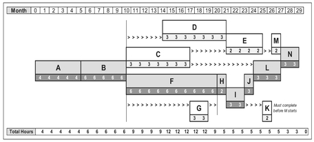
Figure 6.3 Resource Profile Smoothing Using Activity Float Around the Critical Path

Figure 6.4 Critical Path Accelerated by Removing Activities
In some instances, we may find that the Critical Path is ‘not good enough’ (i.e. too long) to meet the business requirement. We may have to resort to increasing resources to accelerate the Critical Path activities need and take the consequential hit on the cost of doing so. However, we may be able to review the solution we have proposed and plan to remove activities from the Critical Path. For example, in the case of our plan to generate a time-phased estimate, we may conclude that we can dispense with the need for a Bottom-up Baseline Estimate and just rely on a Top-down Estimate. This in effect may be sacrificing quality for schedule (and cost as a by-product). Figure 6.4 shows such an accelerated plan with a revised Critical Path.
Here we have removed the three activities that relate to creating Bottom-up Estimates for the Baseline condition and for Risk, Opportunity and Uncertainty. We have also reduced the planned activity duration for Scheduling and creating the Risk and Opportunity Register. This leaves us with only four potential activity paths: ABCEMN, ABDEMN, ABDHIKMN and ABGHIKMN, of which the first becomes the Critical Path with a duration of 22 days.
6.5 Modelling variable Critical Paths using Monte Carlo Simulation
Until now we have only considered Critical Paths with fixed duration activities ... until we started messing around thinking about changing them as a conscious act. However, in many cases we may not know the exact duration an activity will take as there will be Uncertainty around the potential durations and the estimates of the resource times required. In these cases it would be more appropriate to model the schedule with Uncertainty ranges around our activity durations. This leads us to Monte Carlo Simulation and the generation of variable Critical Paths (literally).
If we accept the principle that we discussed in Chapters 3 and 4, there will be an Uncertainty range around the duration of most, if not all, the activities in the network. This then raises the distinct possibility that the Critical Path may not be totally definitive, and that we might only be able to express that a particular activity path is the Critical Path with a specified level of confidence. This may lead us to having to manage activities that are ‘off’ the supposed Critical Path more closely than if they were on the Critical Path; in other words, give them similar priority or due diligence as we give to definitive Critical Path activities.
Consider Activity Path 4 (ABDHIJLN) from our earlier Table 6.3 and compare it with our Critical Path or Activity Path 7 (ABFHIJLN). There is only one activity difference between them; the former includes Activity D whereas the latter includes Activity F. If our Critical Path Activity F (Create Bottom-up Baseline Estimate) takes two days less than anticipated, but Activity D (Create the Project Schedule) takes two days more to complete, then Activity Path 4 becomes the Critical Path, not Activity Path 7.
We can extend this Uncertainty to other activity durations (Table 6.7).
If we were to run a Monte Carlo Simulation using these Discrete Uniform Distribution Uncertainty Ranges in Table 6.7, we would find that Activity Path 7 is only the Critical Path some 85% of the time. Activity Paths 2–4 are also contenders for the Critical Path as summarised in Table 6.8. This tells us that either we can’t add up, or that 14% of the time
Table 6.7 Uncertainty Ranges Around Activity Durations
| ID | Activity | Min | Mode | Max |
|---|---|---|---|---|
| A | Agree Project ADORE | 4 | 5 | 6 |
| B | Agree SoW | 4 | 5 | 6 |
| C | Create Risk Opp Register | 5 | 7 | 9 |
| D | Create Project Schedule | 5 | 7 | 9 |
| E | Perform Schedule Risk Analysis | 3 | 4 | 5 |
| F | Create Bottom-up Baseline Estimate | 6 | 10 | 14 |
| G | Create Top-down Baseline Estimate | 1 | 2 | 3 |
| H | Profile Estimate | 1 | 1 | 1 |
| I | Perform Validation or Challenge | 1 | 2 | 3 |
| J | Update Bottom-up Baseline Estimate | 1 | 1 | 1 |
| K | Update Top-down Baseline Estimate | 1 | 1 | 1 |
| L | Create Bottom-up ROU Estimate | 2 | 3 | 4 |
| M | Create Top-down ROU Estimate | 1 | 1 | 1 |
| N | Create Estimate Recommendation | 1 | 2 | 3 |
Table 6.8 Critical Path Uncertainty
| Activity Path | Occurrences as Critical Path | Comment | |
|---|---|---|---|
| 7 | ABFHIJLN | 85% | Includes instances of 2 or more joint Critical Paths |
| 4 | ABDHIJLN | 20% | |
| 3 | ABCEMN | 6% | |
| 2 | ABDEMN | 3% | |
| Total | 114% |
we have instances where more than one path is the Critical one. Looking at the paths in detail the only activities that are not covered are G and K, which are the creation and update of the Top-down Estimate.
In Figure 6.5, we can show that if Activity Path 7 exceeds its Most Likely Duration of 29 Days, then it is highly probable that it is the Critical Path, and that instances of it not being the Critical Path are associated with the more optimistic durations.
What we have not considered here is that some of these activities may be partially correlated; a schedule overrun in one activity may be indicative of a schedule overrun in another. We can use the same techniques as we did in Chapter 3.

Figure 6.5 Critical Path Uncertainty
Critical Path Analysis and Monte Carlo Simulation are key components that allow us to perform a schedule assessment of Risk, Opportunity and Uncertainty, commonly referred to as Schedule Risk Analysis (SRA). To complete the SRA, we need to add any activity correlation and, of course any Risks or Opportunities that may (or may not) alter the activity durations or add/delete activities.
6.6 Chapter review
In this penultimate chapter, having recognised the need to plan or schedule, we dipped our feet into the heady world of Critical Path Analysis and we looked at how we can apply some simple logic with Binary Numbers to identify the Critical Path in a network of activities or tasks where we don’t have access to specialist scheduling applications.
We explored the ideas of earliest and latest completion dates which give us an indication of optimistic and pessimistic views of the schedule, which in turn allowed us to mull over how we can use this to get an indication of the impact of schedule variation on cost using the Marching Army Technique from Chapter 4.
Finally, bringing it all back into the world of random numbers, we looked at how we can use Monte Carlo Simulation to give us a view of potential finish dates where the Critical Path and the Critical Path duration are variable. Whilst our example was based on the plan for the estimating process, the principles extend to the project in question to be estimated, and as such forms an essential element of a Schedule Risk Analysis. As we discussed in Chapter 4, Schedule Risk Analysis can be a key component of a Topdown pessimistic perspective on the cost impact of Risk, Opportunity and Uncertainty Analysis.
References
Augustine, NR (1997) Augustine’s Laws (6th Edition), Reston, American Institute of Aeronautics and Astronautics, Inc.
Parkinson, CN (1955) ‘Parkinson’s Law’, The Economist, November 19.