
CHAPTER 7
Simple Examples of Hedging with SOFR Futures
In the first half of the book, we focused on the concepts underlying the SOFR futures and options complex, including the repo market, the construction of SOFR, and the specifications and characteristics of SOFR futures and options. In the second half of the book, we focus on practical applications of SOFR futures and options, with an emphasis on specific, worked examples.
In general, SOFR futures and options provide a useful way to manage SOFR risk. But as we consider specific examples, we'll see that it's particularly important in each case to define the terms manage and SOFR risk. For example, one money market fund manager may be interested in minimizing the standard deviation of the net asset value of his fund as of a specific target date, while another money market fund manager may be concerned only with minimizing the downside risk to the NAV of his fund. A corporate treasurer may be interested in using SOFR futures to convert daily rate risk to quarterly rate risk in a cash management program, while a hedge fund trader may be interested in maximizing the Sharpe ratio of a spread trade involving SOFR futures, without knowing the date on which he'll exit the position.
As we work through specific examples, we'll see that the term SOFR risk often entails a collection of risks that differ depending on the context. For example, a bank that wishes to use SOFR futures to convert the risk in a SOFR floating rate note from daily to quarterly may find that 3M SOFR futures provide only a rough approximation of the cash flow dates of the note. On the other hand, if this bank were to use 1M futures to better approximate the cash flows of the FRN, the exposure to rate volatility may increase, owing to the difference between the arithmetic average used in the 1M contract and the geometric average used in the 3M contract.
We'll start with three simple examples involving a corporate treasurer who wishes to convert part of a floating rate balance to fixed.
EXAMPLE 1: CORPORATE TREASURER CONVERTING FLOATING RATE EXPOSURE TO FIXED
Consider a corporate treasurer who had USD 100 million of working capital that he intended to deposit with banks, secured by US Treasuries, starting Wednesday, December 18, 2019, for three months – i.e., up to and including Wednesday, March 18, 2020. As Figure 7.1 suggests, overnight rates had been between 1.5% and 2% in recent months, but these had been trending lower, and there was concern that rates may decline further.
With that in mind, rather than investing the entire amount in overnight repo, he decided he'd like to effectively fix the interest rate he'd receive on half this amount – again, secured by US Treasuries via repo.
To accomplish this, on 18-Dec-19, he purchased three-month Dec19 SOFR futures contracts, expiring in March 2020.
The first thing the treasurer must do is to determine the number of contracts he needs to purchase. He starts with the fact that the CME SOFR futures contract is defined so that the value of a 1 bp change in price is USD 25. He calculates that a 1 bp change in the interest rate earned on a repo investment of USD 50 million over this 91-day period (using an actual/360 day count) is USD 1,263.89. To get this exposure via the three-month SOFR futures market, therefore, he needs to purchase 1,263.89/25 = 50.56 contracts.
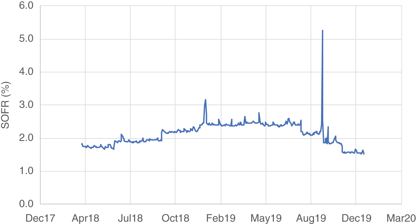
FIGURE 7.1 SOFR
Source: Authors, from Fed data (https://www.newyorkfed.org/markets/reference-rates/sofr) Disclaimer: These reference rate data are subject to the Terms of Use posted at newyorkfed.org. The New York Fed is not responsible for publication of the reference rate data by the Authors and Wiley, does not endorse any particular republication, and has no liability for your use.
In other words:

where the actual sensitivity of a 3M SOFR futures contract is USD 25 by construction; and the desired sensitivity is 0.01 × (di/360) × notional amount. In this case, di, the actual number of calendar days between the start date of December 18, 2019 (inclusive), and the end date of March 18, 2020 (exclusive), happens to be 91. And since the notional amount is USD 50 million in this case, we have: Desired sensitivity = 0.01 × (91/360) × USD 50,000,000 = USD 1,263.89. So the number of contracts our corporate treasurer needs to purchase is USD 1,263.89 / USD 25 = 50.56.
Let's see how this strategy fared in practice. Let's assume that on 18-Dec-19, the treasurer purchased 50 three-month SOFR futures contracts, expiring in 18-Mar-20, with a purchase price of 98.41. The implied SOFR rate is simply 100 – P = 100 – 98.41 = 1.59%. However, this is not the implied daily rate. To calculate the implied daily rate, we need to determine the single interest rate that would result in a final settlement price for the March 2020 futures contract of 98.41, assuming this rate were constant every day from 18-Dec-19 through 17-Mar-20. As it happens, in this case, that rate is 1.5869%.1
Had the SOFR rate been equal to 1.5869% on each day from 18-Dec-19 through 17-Mar-20, the starting value of USD 50,000,000 million would have increased to USD 50,200,956.00 by 18-Mar-20. But, as seen in Figure 7.2, the actual SOFR rate decreased toward the end of this period, such that, without any hedging, the initial deposit of USD 50 million actually increased to only USD 50,187,105.05 – i.e., USD 13,850.95 less than would have been earned had the daily SOFR rate been 1.5869%.
Given the actual SOFR value shown in Figure 7.2, the final settlement price of the Dec-19 three-month SOFR futures contract was 98.5175 – greater than purchase price by 0.1075. Given that the value of a basis point is USD 25 by construction, and given that the treasurer purchased 50 contracts, this change in the price of the futures contract resulted in a gain for the treasurer of 50 × USD 25 /bp × 10.75 bp = USD 13,437.50.
Adding this gain to the actual account balance of USD 50,187,105.05 results in a combined value of USD 50,187.105.05 + USD 13,437.50 = USD 50,200,542.55 – within USD 413.45 of the figure of USD 50,200,956.00 we calculated earlier.
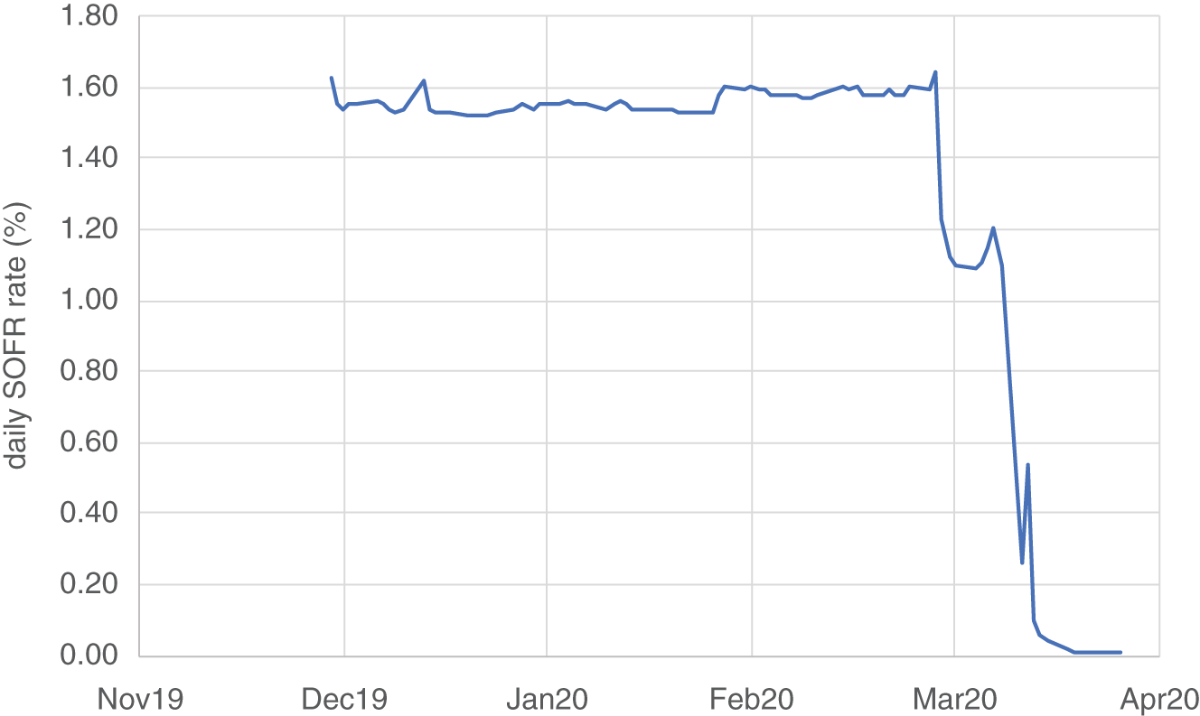
FIGURE 7.2 Actual and implied SOFR values
Source: Authors, from Fed data (https://www.newyorkfed.org/markets/reference-rates/sofr) Disclaimer: These reference rate data are subject to the Terms of Use posted at newyorkfed.org. The New York Fed is not responsible for publication of the reference rate data by the Authors and Wiley, does not endorse any particular republication, and has no liability for your use.
EXAMPLE 2: LOCKING IN AN INTEREST RATE WITH MISMATCHED DATES
What if our corporate treasurer were looking to lock in an interest rate for a somewhat different set of dates? For example, what if the lending period was 2-Dec-19 through 28-Feb-20?2
In this case, the treasurer has a bit of a conundrum, as the Dec-19 three-month SOFR contract covers a somewhat different period, namely 18-Dec-19 (inclusive) through 18-Mar-20 (exclusive). Figure 7.3 illustrates the nature of the problem. The lighter line represents the period for which our corporate treasurer wishes to lock in an interest rate, while the darker line represents the period covered by the Dec-19 three-month SOFR futures contract.
As we can see, there are 12 days at the beginning of the intended lending period that the Dec-19 contract doesn't cover. At the same time, the Dec-19 contract covers an additional 12 business days that are outside of the treasurer's intended lending period. This is no longer a simple date-matching exercise. In this example, we need to make some additional assumptions.
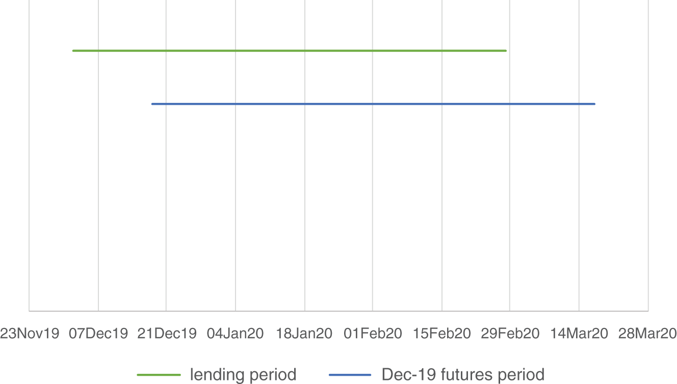
FIGURE 7.3 Intended lending period and period covered by Dec-19 3M SOFR futures
Source: Authors
When dealing with overnight rates, one of the most potentially important events is FOMC meetings. As it happens, there were a few FOMC meetings scheduled during the treasurer's lending period: 11-Dec-19, 29-Jan-20, and 18-Mar-20. So one assumption our corporate treasurer might make is the same assumption made when constructing a Term SOFR rate (as discussed in Chapter 8) – namely, that the term structure of daily SOFR rates can be assumed to be a stepwise function, with each step corresponding to a scheduled FMOC meeting. In this case, we'd have three steps:
- From the beginning of the lending period, 2-Dec-19 through the first FOMC meeting on 11-Dec-19
- From the day after the December 11 FOMC meeting through the second scheduled FOMC meeting on 29-Jan-20
- From the day after the second meeting through to the end of the lending period on 29-Feb-20 (or through 18-Mar-20 when dealing with the three-month SOFR futures contract)
If we're going to make this assumption, we need to find some means of identifying the height of each step in our step function. In particular, we have three unknowns – the heights of our three steps – so it would be ideal if we had three observations we could use to identify these unknown step values.
As it happens, we can use the prices of the Dec-19, Jan-20, and Feb-20 one-month SOFR futures contracts as of 2-Dec-19, in this case 98.37, 98.375, and 98.425, respectively (using settlement prices).
To see the way in which fitted SOFR values can be obtained, consider Table 7.1.
TABLE 7.1 Fitting a stepwise rate curve to one-month SOFR futures prices
Source: Authors
| 1M Dec | 1M Jan | 1M Feb | |
|---|---|---|---|
| fitted SOFR | 1.6300 | 1.6250 | 1.5750 |
| fitted futures prices | 98.37 | 98.37500001 | 98.42500001 |
| settle price | 98.37 | 98.375 | 98.425 |
| (fitted price – settle price)^2 | 1.07776E-13 | 3.44146E-13 | 4.93929E-13 |
In the fourth row, we show the settlement price of each contract. On the fifth row, we show the squared difference between the settlement price and the fitted price, where the fitted price is calculated from the fitted piecewise step function, with the heights of the three steps as the independent variables. More specifically, we choose the heights of the three steps to minimize the sum of squared differences between the actual settlement prices and the fitted prices derived from our fitted, stepwise overnight rate curve.
As can be seen in Table 7.1, we obtain a nearly exact fit with this method, with the resulting rate curve shown in Figure 7.4.
In theory, we could have used the Dec-19 three-month SOFR futures contract to help fit our stepwise rate curve. But in this case, we thought it might be useful to see how closely the fitted price of this contract matched the settlement price on 2-Dec-19. In this case, the settlement price was 98.395, and the fitted price was 98.397. In our view, this difference of 0.002 is quite encouraging, suggesting consistency across the settlement prices of these futures contracts and our fitted stepwise rate curve.
Having built an assumed rate curve, we're in a position to calculate the relative sensitivities of the ending value of our three-month corporate deposit and our hedging instrument – in this case, the Dec-19 three-month SOFR futures contract.
If we bump our fitted curve higher by 1 bp, the ending value of our three-month deposit increases from USD 50,197,252.27 to USD 50,198,479.22, assuming an initial deposit of USD 50,000,000 – a gain of USD 1,226.95. The corresponding change in the price of the three-month Dec-19 SOFR futures contract is 0.01004. Given a point value of USD 2,500, the number of futures contracts required to equate the risk in this case is USD 1,226.95 / (0.01004 × USD 2,500) = 48.88.

FIGURE 7.4 Fitted stepwise overnight SOFR curve
Source: Authors
Our corporate treasurer could round to 49 contracts without introducing much error. But for the sake of discussion, let's assume that he again fixed the number of futures at 50 and solved for the amount of the initial deposit he's going to lock in via futures. In this case, the figure is USD 51,141,741.
Note that the loan period targeted by the corporate treasurer is 89 days – slightly less than 90 days. So it's not surprising that the sensitivity of the ending loan value is such that more than USD 50 million in initial deposit is required to match the sensitivity of a 50-lot position in three-month SOFR futures contracts.
Let's see how this hedge performed in practice. The actual path of SOFR is shown along with our fitted curve in Figure 7.5.
Note that the actual SOFR rate decreased considerably relative to the overnight forward rates along our fitted curve, particularly toward the end of our lending period. As a result, the terminal value of the loan was only USD 51,336,755.08 – i.e., USD 6,742.88 less than our corporate treasurer was trying to lock in.
The final settlement price of the three-month SOFR futures contract was 98.5196, for a gain of 0.1246. Given a position size of 50 contracts and a point value of USD 2,500, this results in a gain of 50 × USD 2,500 × 0.1246 = USD 15,575.
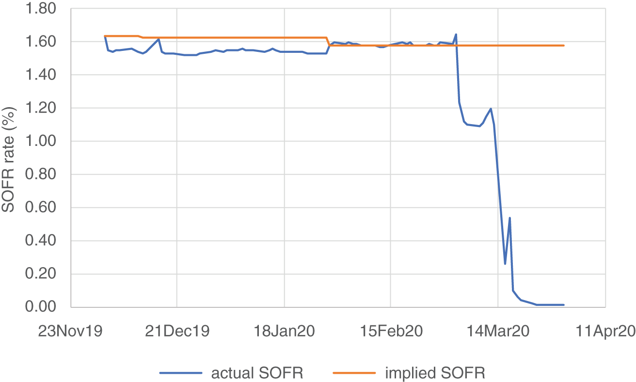
FIGURE 7.5 Fitted stepwise overnight SOFR curve and actual realized SOFR values
Source: Authors
In this case, the gain on the long position in the three-month futures contract was more than twice the shortfall in the ending balance of the deposit relative to the amount the treasurer was trying to lock in. So the futures hedge was helpful, but we can see that there is a fair amount of date mismatch risk when dealing with lending periods that don't match with the periods covered by the futures contract.
In this example, we assumed our corporate treasurer simply held the Dec-19 futures contract until expiration on 18-Mar-20. But in practice, someone in this position typically would be well-advised to sell the futures contract at the prevailing market price at the end of the lending period, since the additional days beyond the lending period are really just introducing noise.
In this case, the settlement price of the Dec-19 three-month SOFR futures contract on 28-Feb-20 was 98.47. Had the treasurer sold the futures hedge at this price, his gain would have been 0.075, resulting in a financial gain of USD 2,500 × 50 × 0.075 = USD 9,375. In this case, the gain on the futures still exceeds the loss of interest on the deposit by a considerable amount – but not by nearly as much as would have been the case in the event the treasurer held the position until expiration, since in this case the price of the Dec-19 futures contract continued to increase between the end of the deposit period (28-Feb-20) and the expiration of the futures contract on 18-Mar-20.
EXAMPLE 3: USING ONE-MONTH SOFR FUTURES AS A HEDGING ALTERNATIVE
In the previous case, the date of the single three-month SOFR futures contract didn't align perfectly with the reference period. In this case, we'll switch to one-month futures in an attempt to construct a more precise hedge.
As before, our corporate treasurer wishes to hedge half of his USD 100 million in overnight deposits from 2-Dec-19 through 28-Feb-20.
Using the term structure of overnight forward rates fitted in the previous example, we calculate that the treasurer's deposit of USD 50 million would grow to USD 50,190,659.93 if he could lock in all the overnight forward rates along this curve. The column, labeled “base curve” in Table 7.2, shows the sizes to which the deposit would grow by various dates in the event the overnight forward rates could be locked in. The next column to the right, labeled “bumped curve,” shows the sizes to which the deposit could grow if the term structure of overnight forward rates were bumped higher by one basis point. The difference between these two values is shown in the next column to the right.
The next column, labeled, “difference,” shows the difference per period. In other words, USD 403.27 of this cumulative difference accrues during the first period; another USD 432.26 of this difference accrues during the second period; and the remaining USD 391.42 accrues during the final period.
The next column in the table shows the basis point values for the one-month contracts considered in this example: Dec19, Jan20, and Feb20. As these are all one-month contracts, the basis point value in each case is USD 41.67.
The next column shows the ratio of the difference per period to the basis point value of each futures contract. This ratio gives us the number of futures contracts we should purchase in order to hedge the size of our deposit. Finally, in the column to the right, we show the actual integer number of each contract to be used in the hedge.
TABLE 7.2 Calculations for a hedge of a simple deposit using one-month SOFR futures
| Base Curve | Bumped Curve | Difference | Difference per Period | Futures BPV | Contracts | Rounded | |
|---|---|---|---|---|---|---|---|
| deposit on 2-dec-19 | 50,000,000.00 | 50,000,000.00 | 0.00 | ||||
| deposit on 31-dec-19 | 50,065,693.08 | 50,066,096.35 | 403.27 | 403.27 | 41.67 | 9.678 | 10 |
| deposit on 31-jan-20 | 50,135,873.19 | 50,136,708.72 | 835.53 | 432.26 | 41.67 | 10.373 | 10 |
| deposit on 28-feb-20 | 50,197,324.48 | 50,198,551.43 | 1,226.95 | 391.42 | 41.67 | 9.393 | 9 |
How Did This Hedge Perform in Practice?
As we saw above, the actual SOFR values toward the end of this period were far below the overnight forward rates as of 2-Dec-19. As a result, the deposit would have grown only to USD 50,190,659.93 had it been left unhedged – a shortfall of USD 6,664.55 relative to the value consistent with the overnight forward rates as of 2-Dec-19.
At the same time, our futures hedge returned USD 6,379.68. With this gain, our net shortfall was reduced to USD 284.88 – a hedging error of 4.3%.
Note that the hedging error in this case was much lower than the hedging error in the previous case, in which the date mismatch between the interest period on the deposit and the reference period of the futures contract was material.
LESSONS TO BE LEARNED FROM THESE THREE SIMPLE EXAMPLES
From these three simple examples, we take away a few key lessons.
Hedge Ratios Are Relative Sensitivities
In all three examples, the thing we wanted to hedge (our hedge target) was the size of our cash balance at the end of the reference period. And the instruments we used to hedge were futures contracts: a three-month contract in the first two examples and a collection of one-month contracts in the third example.
But in each case, the strategy for calculating our hedge ratios was the same: to identify a state variable and then to make sure the sensitivity of our futures hedge to changes in that state variable were the same as the sensitivity of our hedge target to changes in that state variable. In the first example, the state variable was simply the final settlement rate of the futures contract (i.e., 1 – the final settlement price of the futures contract), since that rate determined both the gains from our futures contract and the size of our ending cash balance.
In the second example, the state variable was a parallel shift in the fitted yield curve. In particular, we did our best to make sure that a one basis point bump in the term structure of overnight forward rates produced a sufficient gain on our futures position to offset any shortfalls experienced in our ending cash balance. This was the approach taken in the third example, as well – though in the third example we had to contend with three hedging instruments rather than one.
But in each case, the strategy is first to identify a useful state variable and then to create a portfolio of futures contracts for which the change in net present value due to a change in the state variable offsets the change in the value of our hedge target (the ending value of our cash balance in these examples) due to the same change in the value of the state variable.
Dates Matter
In the first example, the reference period of our hedge corresponded with the reference period of our single hedge instrument, a three-month SOFR futures contract. And we saw that the performance of the hedge was relatively good.
In the second example, the reference period of our three-month futures contract didn't correspond particularly well with the reference period of our hedge, and despite our best efforts the performance of the hedge was relatively poor.
In the third example, we were able to regain a close correspondence between the reference period of our hedge and the reference period of our hedging instruments by using a collection of one-month futures contracts rather than a single three-month futures contract. And here again, we saw that the performance of the hedge was relatively good.
It's not always possible to choose hedging instruments with reference periods that correspond closely to the reference period of the target you wish to hedge. For example, if our deposit period ran from 15-Jan-20 through 15-Apr-20, neither a single three-month futures contract nor a collection of one-month futures contracts would provide a close correspondence between the reference period of our hedge instrument and the reference period of our target hedge. In those cases, we do our best, but we need to acknowledge that the performance of our hedge simply isn't likely to be as good in this instance as it would be otherwise.
Assumptions Matter
In the first example, we didn't need to make any assumptions about the behavior of the term structure of overnight forward rates, since the reference period of our hedge target was the same as the reference period of our hedge instrument.
But in the second and third examples, we needed to make assumptions, even if we weren't explicit about these assumptions at the time. In particular, in both examples, we assumed that the term structure of overnight forward rates moved in parallel, allowing us to assess relative sensitivities of our hedge target and hedge instruments simply by bumping the curve.
In practice, nobody believes this is truly the way the term structure moves. However, it may be a useful assumption in certain circumstances. More to the point, it may be a relatively useful assumption to make if the cost of making a more realistic assumption is likely to be large relative to the improved performance of the hedge under that assumption.
For example, in Chapter 8, we'll propose a method for precisely hedging forward CME Term SOFR values using a portfolio of one-month and three-month futures contracts. The assumptions underlying this approach may be more realistic (or at least less restrictive), though they do come with some additional computational costs, as we'll see in the next chapter.