CHAPTER 8
Hedging the CME Term SOFR Rate
At some level, the secured overnight financing rate is an elegant concept, as it represents the most basic building block for yield curves. But as we have described in Chapter 3, there are a significant number of market participants for whom SOFR isn't ideal. For example, many corporate treasurers appreciate knowing the cash flows of their loans well in advance of those cash flow payment dates. And for these people, a plan vanilla SOFR loan simply isn't an attractive arrangement, due to the fact that the ultimate size of each interest payment is known only shortly in advance of the interest payment date.
In theory, secured financing rates for specific terms could be constructed the way the Fed constructs the secured overnight financing rate – i.e., by averaging each day the interest rates reported for repo transactions for specific terms, such as one month, three months, and six months. In practice, however, this is seen as problematic, as the volume of daily transactions with terms of three months, six months, etc., is considered to be insufficient for this purpose.
As an alternative, someone could organize a process in which banks are asked each day to provide the rates at which they would be willing to enter into repo transactions of various terms. And then these rates could be averaged and published at the same time each day. Of course, the problem with this approach is that regulators would be unwilling to sanction a process that they believe could be manipulated the way the LIBOR rate-setting process was manipulated.
So the market found itself facing a bit of a conundrum. The LIBOR rigging scandal precludes the use of a survey to determine secured term financing rates. And yet there aren't enough secured term repo transactions reported each day to create a robust averaging process.
In an attempt to address this issue, the Chicago Mercantile Exchange introduced Term SOFR,1 for terms of one month, three months, six months, and twelve months. Term SOFR attempts to address the conundrum by converting a set of transactions reported in the SOFR futures market into a yield curve and then using this yield curve to calculate the values of spot rates with the desired tenors.
THE TERM SOFR METHODOLOGY
The inputs to the CME Term SOFR calculations are prices of one-month and three-month SOFR futures contracts. In particular, the methodology uses the first thirteen one-month contracts and the first five three-month contracts.
If the all the overnight values along the SOFR curve are allowed to differ from one another, then in general there will be an infinite number of combinations that will be exactly consistent with the prices of the eighteen futures contracts used as inputs to the process. More specifically, the yield curve will be underidentified – i.e., there won't be enough information to determine which of these yield curves should serve as the basis for calculating term rates.
In theory we could select a curve from this infinite collection of curves based on an additional criterion. For instance, we might select the smoothest of these curves according to some definition of smoothness. For example, in many applications the smoothness of a curve is measured by the integral of the square of the second derivative along the curve. In the case of SOFR curves we could define an analogous concept by summing the squared butterfly spreads along the term structure of overnight forward rates.2
THE CME TERM SOFR OBJECTIVE FUNCTION
However, the CME decided to take a different approach to the problem of an under identified yield curve. More specifically, the CME introduced an additional assumption – namely, that the term structure of overnight forward rates consists of a step function, with FOMC meeting dates defining the positions of these steps. In other words, the CME assumes that all the overnight forward rates between any two FOMC meeting dates have identical values. For example, all the overnight forward rates between the January and March FOMC meetings are presumed to have the same values, and all the overnight forward rates between the March and May FOMC meetings are presumed to have the same values. The values of the forward rates in each segment generally differ from the values of the forward rates in other segments, but the values of the forward rates within each segment are presumed to be identical.
With this assumption, the degrees of freedom in the problem decline from a couple hundred to something on the order of 10 – and certainly to a number smaller than the number of futures contracts used in the process. As a result, this assumption takes us from having a yield curve that is underidentified to having a yield curve that is overidentified. In other words, our degrees of freedom are now fewer than the number of futures contracts whose prices we wish to match. In general, we won't be able to match all the input futures prices exactly.3
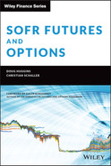
In order to identify specific, unique values for the heights of the steps in their stepwise yield curve, the CME specifies that step values should be chosen so as to minimize the sum of squared differences between the futures prices observed in the market and the futures prices produced by the fitted term structure of overnight forward rates. In particular, the CME (October 2021) chooses the heights of the steps in their stepwise yield curve so as to minimize the value of the objective function
where
- N is the number of steps.
- Φ is the vector of step values,
 , for
, for 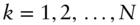 .
.  is the price of the mth one-month SOFR futures contract.
 is the fitted price of the mth one-month SOFR futures contract.
 is the price of the qth three-month SOFR futures contract.
 is the fitted price of the qth three-month SOFR futures contract.
 is the weight associated with the mth one-month futures contract.
 is the weight associated with the qth three-month futures contract.
In theory, this criterion should be sufficient for identifying a stepwise yield curve from which to calculate term SOFR rates each day. But in practice, the stepwise yield curve fitted in this manner may exhibit undesirable characteristics at times. For example, depending on the FOMC meeting dates and futures expiration dates, it's possible this process could produce a curve in which the variability between successive steps is implausibly large.
In an attempt to prevent this, the CME adds an additional regularity condition – in this case a penalty function – to equation 8.1. In particular, this penalty function is given by the sum of squared differences between adjacent steps weighted by a number, λ, that scales this penalty function. As a result, the actual objective function used by the CME to determine the values of the steps in its stepwise yield curve is given by
where λ is the weight associated with the penalty function.
If the value of λ is 0, then the penalty function has no effect whatsoever on the fitted step values. On the other hand, if the value of λ is large, then the fitted term structure of overnight forward rates will be horizontal.
Of course, the calculated term SOFR rates are a function of the fitted yield curve, so they're also a function of the value of λ. For example, Figure 8.1 shows the fitted 6M term SOFR rate as a function of λ, using data for 27-Jan-22.
As we can see from the figure, large values of λ can have very significant implications for the term SOFR rates published by the CME – on the order of 30 basis points for very large values of λ.
According to the CME, the value of λ currently is set to ![]() . As the number of scheduled FOMC meetings over the course of a year is typically eight or nine, the typical value of λ appears to be on the order of
. As the number of scheduled FOMC meetings over the course of a year is typically eight or nine, the typical value of λ appears to be on the order of ![]() , roughly 0.33. In the present example, that's enough to increase the 6M term SOFR rate by slightly more than half a basis point relative to the term SOFR rate calculated when
, roughly 0.33. In the present example, that's enough to increase the 6M term SOFR rate by slightly more than half a basis point relative to the term SOFR rate calculated when ![]() .
.
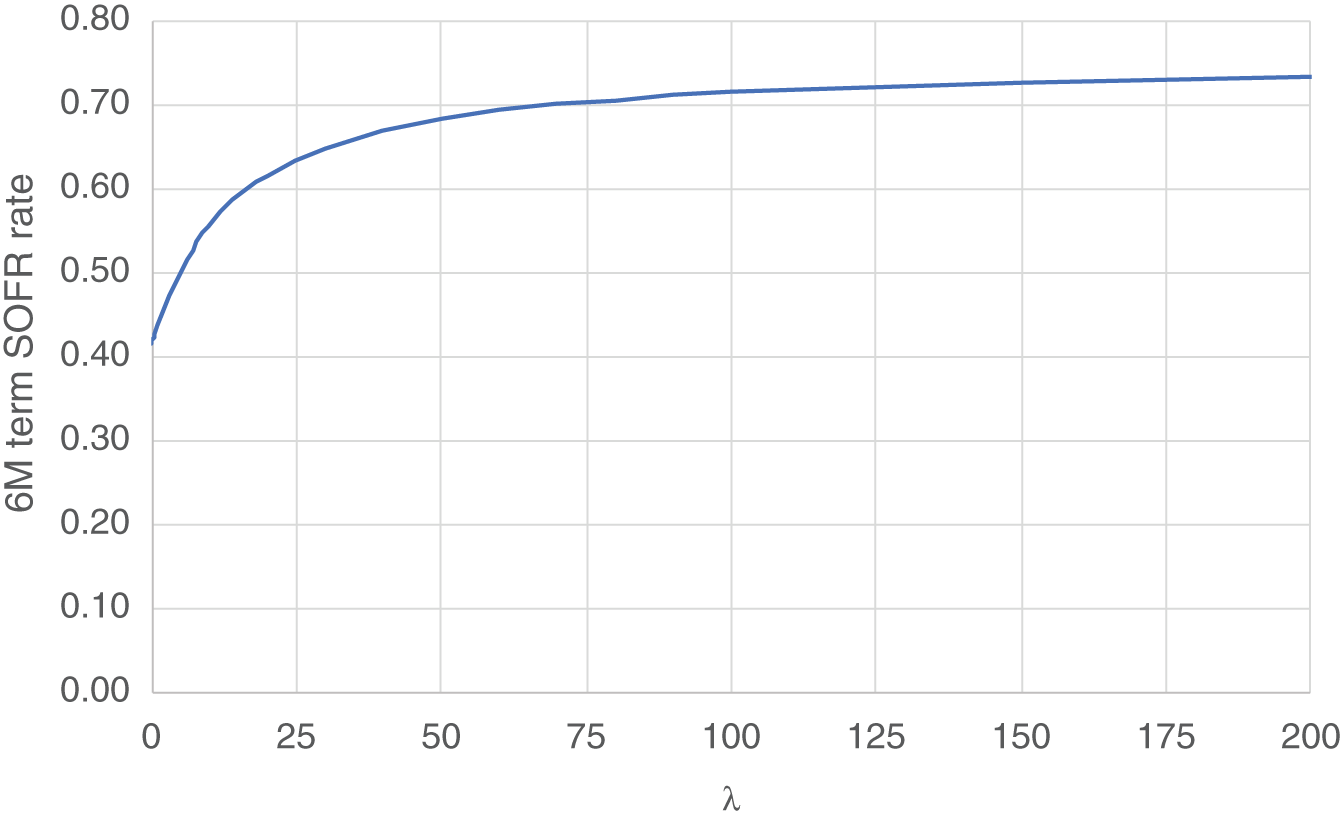
FIGURE 8.1 6M term SOFR rate as a function of λ for 27-Jan-22
Source: Authors
Half a basis point doesn't seem like a large number. Of course, when it's multiplied by hundreds of millions or even billions of dollars, it starts to add up. And as the yield curve tends to be upward-sloping more often than downward-sloping, our sense is that the inclusion of this penalty function probably imparts an upward bias to term SOFR rates, favoring lenders and disfavoring borrowers. To be fair, however, we haven't analyzed this issue in any great detail, and more work would be required before we could determine whether this penalty function in fact does impart a systematic bias in published term SOFR rates.
This analysis does beg a few questions, however: Who chooses the value of λ? What criteria are used in making this choice? Is this choice an objective decision or a subjective decision? To what reviews is this decision subject, and are these reviews made public?
We don't mean to suggest there's anything amiss in this process. But for borrowers and lenders using CME Term SOFR rates as references, a lot of money is at stake, and we believe the market would benefit from even greater transparency into this issue.
OBTAINING FUTURES PRICES TO USE AS INPUTS TO THE TERM SOFR MODEL
In the preceding discussion, we simply assumed that an appropriate set of futures prices was available to serve as inputs to the term SOFR calculation methodology. In practice, the situation isn't that simple.
The CME has produced an involved methodology for determining each day's input price for each futures contract. This methodology isn't entirely straightforward, and the written explanation provided by the CME (October 2021) isn't sufficiently precise for their calculations to be checked and/or replicated by typical market participants (even if these market participants had access to all the necessary data).
But the gist of the approach is as follows (see also Figure 3.2):
- The trading day from 7:00 a.m. to 2:00 p.m. Chicago time is divided into 14 intervals, each of 30-minute duration.
- In each time interval, the CME will compute a volume-weighted average price (VWAP) for each of the 18 futures contracts used to produce the term structure of overnight forward rates.
- The CME also will choose a random time during each of these 14 intervals to observe the bid–ask spread for each contract.
- If the VWAP for each futures contract is within the observed bid–ask spread during an interval, then the VWAP is recorded as the futures price for that contract during that interval. If the VWAP for a futures contract is greater than the ask price (lower than the bid price), then the ask price (bid price) will be recorded as the futures price for that contract for that interval.
- For each futures contract, the reference price for that day will be the volume-weighted average of the 14 prices recorded during each of the 14 time intervals, where the weights are the aggregate volumes of all the futures contracts traded in that interval as a fraction of the total volume of these 18 futures contracts during the day.
There are some further caveats, for example, to account for intervals in which no trading occurred – but this is the gist of the approach.
HEDGING TERM SOFR EXPOSURE
At the end of Chapter 2, we presented an approach to hedge with a portfolio of futures against changes in the step function determining a term rate. This relatively simple method could be considered as an approximate hedge for the CME Term rate as well. However, in case a more precise hedge of the CME Term rate is desired, the more complex method described below seems advisable. After presenting this method and experiencing the issues involved, we'll conclude that there is a tradeoff between the precision and the ease of the hedge.
Consider someone who borrows money for one year and who agrees to pay the 3M term SOFR rate at the end of month 3, month 6, month 9, and month 12. The first term SOFR rate would be specified at the start of the loan, so there is no need to hedge this rate. But in theory we could hedge the three remaining interest payments:
- A payment at the end of month 6 of the 3M CME Term SOFR rate published at the end of month 3
- A payment at the end of month 9 of the 3M CME Term SOFR rate published at the end of month 6
- A payment at the end of month 12 of the 3M CME Term SOFR rate published at the end of month 9.
Let's assume that our borrower wishes to use SOFR futures to minimize the standard deviation of the sum of these random interest payments. What should he do?
A PRECISE APPROACH TO HEDGING CME TERM SOFR EXPOSURE
Consider a situation in which we're given a portfolio of stocks but without being told the quantities in which each individual stock is being held. But imagine further than we could learn the change in the value of the portfolio for a one-unit change in the value of each instrument. In that case, we could hedge the short-term change in the value of this portfolio by selling each stock in proportion to the sensitivity of the portfolio value to a change in the price of this stock. For example, if the portfolio increases in value by USD 100 when the price of IBM stock increases by one dollar, we should sell 100 shares of IBM as part of our hedging strategy. And if the value of the portfolio decreases by USD 50 when the price of Coca-Cola stock increases by one dollar, we should buy 50 shares of Coca-Cola as part of our hedging strategy.
We can apply a similar approach when dealing with our term SOFR exposures. For example, imagine that the 3M CME Term SOFR rate corresponding with our next interest payment increases by 5 bp when the price of the Dec22 one-month SOFR futures contract decreases by 10 bp. And let's imagine that the size of our loan is USD 10 million, such that a 5 bp increase in a quarterly interest rate corresponds to an increase in our interest expense of USD 10,000,000 × 0.0005 × (90/360) = USD 1,250. To hedge this, we want the value of our position in the Dec22 one-month SOFR futures contract to increase by USD 1,250 in response to a 10 bp decrease in the price of the Dec22 contract. Since a 1 bp price change is worth USD 41.67 per contract, a 10 bp price change is worth USD 416.70 per contract. So in order to experience a change in the value of our position equal to USD 1,250, we need to sell USD 1,250 / USD 416.70 = 3 Dec22 one-month futures contracts as part of our hedge portfolio. By repeating this calculation for each of the futures contracts that determine the value of the 3M CME Term SOFR rate, we can construct a portfolio that locally will hedge the exposures to CME Term SOFR rates in our loan. We say that our hedge portfolio will hedge the exposure locally because the sensitivities in this example may change as futures prices change and as time passes. We need to repeat these calculations regularly and adjust the positions in our hedge portfolio accordingly.
Let's consider a specific example in greater detail.
Consider a two-year loan, arranged on 27-Jan-22, which pays three-month CME Term SOFR rate every three months until the maturity of the loan, in two years. Assume that the amount of the loan is USD 100 million.
The first interest payment will be due on Friday, 27-Apr-22. But as the rate applying to the first period is known at the time the loan is arranged, this isn't something we can hedge.
The second interest payment will be due on Wednesday, 27-Jul-22, and as it will be set at the end of April, we can hedge this rate and the corresponding payment. The forward value as of 27-Jan-22 for this CME Term SOFR is 0.54850%, and the forward value on 27-Jan-22 of the associated interest payment4 is USD 136,992.80.
The strategy for hedging this payment will be the same as in the simple example above involving shares of IBM and Coca-Cola. More specifically, we'll follow three steps:
- Build a stepwise term structure of overnight forward rates, with the discontinuities corresponding to FOMC dates, just as the CME does when calculating CME Term SOFR values.
- Calculate the sensitivity of the forward-starting CME Term SOFR – and hence of the interest payment to be hedged – to a change in the price of each futures contract.
- Construct a hedge portfolio of futures contracts so that the sensitivity of the value of the hedge portfolio to a change in the price of each futures contract is the opposite of the sensitivities calculated in step 2.
When we're done, the value of the combined position – i.e., the size of the payment being hedged plus the value of the hedge portfolio – should be insensitive to changes in the prices of any of the 18 futures contracts. In that case, we will have succeeded in immunizing the size of the payment from changes in the prices of any of the 18 futures contracts.
To see the calculations in greater detail, consider Table 8.1.
TABLE 8.1 Calculations for hedge of 3M term SOFR starting 27-Apr-22, as of 27-Jan-22
Source: Authors
| # | Futures Identifier Code | Settlement Price | Payment (− 5 bp) | Payment (+ 5 bp) | Payment Difference | Value of 10 bp Change in Futures Price | Number Futures to Sell | Number of Futures to Sell (rounded) |
|---|---|---|---|---|---|---|---|---|
| 1 | SERF2 | 99.95 | 137,012.37 | 136,973.24 | −39.14 | 416.70 | −0.094 | |
| 2 | SERG2 | 99.95 | 137,144.61 | 136,840.99 | −303.62 | 416.70 | −0.729 | |
| 3 | SERH2 | 99.805 | 136,669.14 | 137,316.46 | 647.31 | 416.70 | 1.553 | 1 |
| 4 | SERJ2 | 99.655 | 136,106.57 | 137,878.98 | 1,772.41 | 416.70 | 4.253 | 4 |
| 5 | SERK2 | 99.485 | 132,868.35 | 141,117.34 | 8,248.99 | 416.70 | 19.796 | 20 |
| 6 | SERM2 | 99.37 | 133,965.39 | 140,020.34 | 6,054.95 | 416.70 | 14.531 | 14 |
| 7 | SERN2 | 99.265 | 135,744.63 | 138,240.96 | 2,496.33 | 416.70 | 5.991 | 6 |
| 8 | SERQ2 | 99.155 | 137,035.21 | 136,950.38 | −84.83 | 416.70 | −0.204 | |
| 9 | SERU2 | 99.105 | 137,023.18 | 136,962.41 | −60.78 | 416.70 | −0.146 | |
| 10 | SERV2 | 98.995 | 136,994.69 | 136,990.90 | −3.79 | 416.70 | −0.009 | |
| 11 | SERX2 | 98.905 | 136,992.89 | 136,992.73 | −0.17 | 416.70 | 0.000 | |
| 12 | SERZ2 | 98.825 | 136,992.75 | 136,992.83 | 0.08 | 416.70 | 0.000 | |
| 13 | SERF3 | 98.76 | 136,992.77 | 136,992.83 | 0.06 | 416.70 | 0.000 | |
| 14 | SFRZ1 | 99.95 | 137,071.22 | 136,914.38 | −156.83 | 250.00 | −0.627 | |
| 15 | SFRH2 | 99.565 | 134,466.31 | 139,519.48 | 5,053.17 | 250.00 | 20.213 | 20 |
| 16 | SFRM2 | 99.205 | 136,350.04 | 137,635.60 | 1,285.56 | 250.00 | 5.142 | 5 |
| 17 | SFRU2 | 98.93 | 136,994.12 | 136,991.48 | −2.65 | 250.00 | −0.011 | |
| 18 | SFRZ2 | 98.72 | 136,992.78 | 136,992.82 | 0.04 | 250.00 | 0.000 |
In the left-most column, we have the identifier codes for the 13 one-month SOFR contracts and the 5 three-month futures contracts used in this exercise. In the column immediately to the right, we have the settlement prices of these futures contracts as of 27-Jan-22. In the next column to the right, we have the size of the next payment according to a fitted curve in which the input price of each futures contract has been decreased from its actual value by 5 bp. In the column to the right of that, we have the size of the next payment according to a fitted curve in which the input price of each futures contract has been increased from its actual value by 5 bp. The next column to the right shows the difference between the values in the two columns immediately to the left. In other words, the values in this column show the change in the size of the next payment due to a 10 bp change in the input price of each futures contract. Now we need to compare the values in this column to the value of a 10 bp change in the futures rate associated with each contract. These are shown in the next column to the right. As a reminder, the value of a 10 bp change is 10 × USD 41.67 = USD 416.70 for the case of a one-month SOFR futures contract and 10 × USD 25 = USD 250.00 for the case of a three-month SOFR futures contract.
The next column to the right shows the ratio of the change in the value of each payment to the change in the value of each futures contract, due to a 10 bp change in the futures rate of each futures contract. The values in this column show the number of futures contracts we should sell to construct a portfolio that hedges the size of our next random interest payment, which is tied to the random value of the CME Term SOFR. The final column on the right shows these values rounded to the nearest integer.
Let's consider the composition of this hedge portfolio before rounding. The net number of one-month futures contracts we're to sell is 45, while the net number of three-month futures contracts we're to sell is 25. Let's think whether these figures make sense, even to a first approximation.
If the reference period of a one-month contract is 30 days, then a basis point value of USD 41.67 corresponds to a notional amount of USD 5 million. So if we're hedging a notional amount of USD 100 million for a reference period of one month, we'd expect to sell 100/5 = 20 one-month contracts. And if we hedge a notional amount of USD 100 million for a reference period of three months, we'd expect to sell a total of 3 × 20 = 60 contracts – again, assuming we're using one-month SOFR contracts.
On the other hand, if we were using three-month SOFR futures contracts, and if the reference period were 90 days, then a basis point value of USD 25 corresponds to a notional amount of USD 1 million. So if we're hedging a notional amount of USD 100 million for a reference period of three months, we'd expect to sell 100 contracts – again, assuming we're using three-month SOFR futures.
In our hedge portfolio, we're using a combination of one-month and three-month SOFR futures contracts. In particular, we're using 45 one-month contracts and 25 three-month contracts. Since 60 one-month contracts have the hedging power of 100 one-month contracts, we can convert contracts in a mental accounting exercise. Since 25 three-month contracts have the hedging power of 25 × 60/100 = 15 one-month contracts, our combined hedge portfolio has the hedging power of 45 + 15 = 60 one-month contracts, just as our intuition suggested it should have.
On the other hand, we also can convert the hedging power of our one-month contracts to the hedging power of three-month contracts at the same ratio – i.e., 60 one-month contracts for every 100 three-month contracts. In that case, our 45 one-month contracts have the hedging power of 75 three-month contracts. And adding this to the actual position of 25 three-month contracts gives us a combined hedging power equal to 100 three-month contracts – again, in accordance with our intuition.
So our hedge portfolio appears to provide the overall hedging power we'd expect. And looking carefully at Table 8.1, we can see that the composition of this hedge is focused on the period covered by our next random interest period – 27-April-22 through 27-Jul-22.
To get a feel for the performance of this hedge, we can manipulate the term structure of overnight forward rates and see whether our futures hedge portfolio offsets the changes in the forward Term SOFR value and the associated size of our next random interest payment.
For example, let's assume that all the overnight forward rates starting with the 16-Mar-22 FOMC date were to increase from their 27-Jan-22 fitted values by 25 bp. Then the forward Term SOFR value would increase from 0.54195% to 0.79222% – an increase of 25 bp. And the associated interest payment would increase from USD 136,992.80 to USD 200,256.20 – an increase of USD 63,263.40. At the same time, the value of our futures hedge portfolio would increase by USD 62,830.08 – within USD 433.32 of the increase in the value of our interest payment. In this case, the hedge performed to within seven tenths (0.7) of 1%.
If the values of the overnight forward rates after the 16-Mar-22 FOMC instead had decreased by, say, 40 bp, then the value of our interest payment would decrease by USD 101,167.61, which would be largely offset by a loss of USD 99,739.44 in the value of our futures portfolio. In this case, the performance of the hedge was to within 1.4% of target.
PRACTICAL CONSIDERATIONS
To calculate the sensitivity of the forward CME Term SOFR value to the input price of each futures contract, we needed to calculate the first partial derivatives of the forward CME Term SOFR value with respect to the prices of each of the eighteen futures contracts serving as inputs to the CME Term SOFR algorithm. And because there is no closed-form solution for the forward CME Term SOFR value as a function of the futures prices, we needed to calculate these partial derivatives numerically. And because we wanted to obtain a high degree of accuracy, we used central differencing to calculate these partial derivatives, meaning we had to evaluate the objective function and calculate the forward CME Term SOFR value 36 times. And because each evaluation of the objective function required a numerical, nonlinear optimization, we needed to perform 36 of these. And that's just to hedge a single quarterly payment. To precisely hedge all the quarterly payments in a five-year loan would require hundreds of numerical, nonlinear, multidimensional optimizations. This isn't a task for the faint-hearted.
On the other hand, we did the calculations in this example in Excel. These calculations are tedious, and they're cumbersome – but they're also feasible without any special hardware or software. Having said that, we strongly suggest anyone who has a need to perform these calculations regularly and/or for a large loan book invest the time to automate these calculations.
The occasional hedger, who does not require a high degree of accuracy, may want to consider the approximate hedge (of a term rate) described at the end of Chapter 2 as an easier alternative. (See the Excel spreadsheet “Term rate hedge example” accompanying Chapter 2.)
Another issue to consider is the global nature of the algorithm for fitting a term structure of overnight forward rates. Looking carefully at the futures hedge portfolio detailed in Table 8.1, we see that the hedge portfolio contains one lot of the Mar22 one-month contract, even though the reference period for the Mar22 contract ends almost four weeks before the start date of our forward CME Term SOFR. And the hedge contains four lots of the Apr22 one-month contract, even though the overlap between the reference period of this contract and that of our forward CME Term SOFR is only a few days.
To help explain the composition of the hedge portfolio, it's useful to note that the fitted curve in this case is not bootstrapped, and the fitted curve depends on the inputs globally. For example, the curve-fitting algorithm may sacrifice the fit between observed and fitted futures prices in one part of the curve to improve the fit in other parts of the curve. Or the algorithm may allow the curve to become steeper in one region so that the curve can be flatter in another region. Such tradeoffs may be optimal when dealing with a global objective function that contains a global penalty function, but it means that changes in the prices of futures contracts that have no overlap with our CME Term SOFR value can still influence the CME Term SOFR value produced by the algorithm. We see the motivations behind designing an algorithm with this property, but it still makes us a little nervous. And it's certainly something that users need to keep in mind when implementing this curve-fitting methodology.
A bigger concern for us is that the process by which futures input prices are determined is not transparent. In fact, as this process involves collections of bid prices and offer prices taken at 14 random times throughout the day, it's fair to say that the process is opaque by design.
We're also slightly concerned by the fact that the CME Benchmark Administrator (CBA) doesn't make any of the input prices to the algorithm publicly available. We see no reason that this shouldn't be done, and we'd feel more comfortable if the input prices were published each day, along with the intermediate calculations that produced each input price.
The CME Term SOFR algorithm can be changed after consultation, and we understand that, in this event, the CBA will make an effort to inform licensed users of any changes to this methodology. But our view is that these CME Term SOFR values may well become part of the broader financial ecosystem, in which case a much broader community should be informed in advance of any changes to the methodology – and at the same time that licensed users are informed of these changes. For that reason, we'd like for the consultation process and any subsequent announcements regarding changes to CME Term SOFR to be made public.
NOTES
- 1 We appreciate the irony of the label “term secured overnight financing rate.”
- 2 For example, if the term structure of overnight forward rates were as simple as 0.05, 0.04, 0.05, 0.06, 0.04, then this smoothness measure would be given by
 .
. - 3 If the yield curve is such that we are unable to match the prices of all the input futures contracts exactly, it may be tempting to conclude that an arbitrage exists – i.e., that we could obtain riskless profits by trading one set of futures contracts against another. However, this conclusion would be unwarranted. We're unable to reprice our input futures contracts in this case only because of the assumption that the term structure of overnight forward rates is a step function. If we relax that assumption, it will be possible generally to find a curve that reprices all the futures contracts precisely, consistent with the absence of arbitrage. In fact, as discussed, it generally would be possible to find an infinite number of such curves.
- 4 In this exercise, we're calculating partial derivatives numerically, and to use the greatest precision possible, we will not be rounding values as per convention during these intermediate calculations.