
CHAPTER 1
SOFR
THE REPO MARKET
The Secured Overnight Financing Rate (SOFR) is based on data collected from the market for overnight repurchase agreements (i.e., the repo market). A repo transaction is a loan collateralized by a bond, usually of very high quality, such as a US Treasury note. Since a repo agreement is a secured loan, the interest rate associated with a repo transaction is usually lower than interest rates for otherwise similar unsecured loans, such as LIBOR.
This difference also leads to a lower Bank for International Settlements (BIS) risk weighting (e.g., 0% for US Treasuries) and thereby to lower capital costs (Huggins and Schaller 2013, p. 148). Hence, the motivation for the borrower in the repo market is the lower interest rate that can (usually) be obtained with a secured financing. The motivation for the lender in the repo market is the significant reduction of credit risk and a lower cost of capital.
In addition, lenders may be motivated to receive a specific bond as collateral in the repo transaction in order to cover a short position in this bond. The fact that the repo market can be used to cover short positions makes it a vital component of many relative value trades – and therefore the repo rate appears in many relative value relationships and arbitrage equations. For example, the “classical” relative value trade of buying a bond futures contract and selling a bond deliverable into that contract requires covering the short position in the bond until the delivery date of the futures contract. As a result, the repo rate is a direct determinant of the spread between the forward price of the bond and the price of the futures contract. Seen from another perspective, the price of each deliverable bond can be expressed in terms of its implied repo rate – i.e., the repo rate that would be earned by purchasing the bond in the spot market, selling the futures contract, and delivering the bond into the short futures position (Huggins and Schaller 2013, p. 121).
The vital function of the repo market for relative value trading also means that relative value relationships, at times, can exert a significant influence on the repo market. For example, if a futures contract were trading cheap to the cheapest-to-deliver bond, one could buy the futures contract and sell the bond, using the repo market to cover the short position in the bond. This situation often results in traders being willing to lend cash at lower rates in exchange for the cheapest-to-deliver bond as collateral. A borrower of cash in the repo market can then enjoy an especially low rate, provided he secures the loan with the cheapest-to-deliver bond rather than a generic US Treasury. Accordingly, a bond is said to be “special collateral” or “on special” when its repo rate is below the repo rate earned by general collateral. Apart from bonds that are cheapest-to-deliver in futures contracts, specialness tends to occur in bonds for which there are significant short positions, such as new issues and benchmarks (Huggins and Schaller 2013, p. 291).
If the lender of cash in a repo transaction is unable to return the collateral to the borrower at maturity, this is called a failure, which carries penalties. In order to avoid the risk of failures, tri-party repo can be used, where a custodial bank holds the collateral as a third party to the repo transaction. In tri-party repo, no specific bonds can be selected as collateral, so the tri-party repo rate can be considered as a general collateral rate, (almost) without the risk of failure. For this reason, on any given day, the probability distribution for tri-party repo rates tends to be narrower than the probability distribution for bilateral repo rates. On the left tail of the distribution, it excludes special repo rates and any premium charged for the possibility of the counterparty failing.
SOFR: DEFINITIONS AND FEATURES
One can formulate general goals for the task of condensing the overnight repo market into a single number, which is intended to serve as a reference rate for collateralized overnight private sector lending and to replace LIBOR:
- On one hand, the portion of the repo market considered needs to be large enough to be representative, not easily manipulable, and provide enough liquidity even in times of crisis.
- On the other hand, the intended use as a reference rate requires sufficient stability. Given the structure of the repo market, it has at least one inherent source of instability from special bonds, which needs to be excluded from the reference rate as much as possible.
- Given the experience of LIBOR, which motivates the whole exercise, the new reference rate should be based on actual market transactions rather than on surveys of panel members.
The Secured Overnight Financing Rate is the solution suggested by the Alternative Reference Rates Committee (ARRC) and proposed to the Federal Reserve. Figures 1.1, 1.2, and 1.3 summarize the main characteristics of SOFR, which the New York Fed publishes on its website, https://www.newyorkfed.org/markets/reference-rates/sofr, with historical data being available from April 2, 2018.
These definitions and features reflect the status at the time of writing (December 2021). We encourage the reader to monitor the sources mentioned (specifically, Figure 1.2 source) for changes and updates.
| Data input: | TGCR (Tri-Party General Collateral Rate) | Tri-party repo conducted with BNYM (Bank of New York Mellon) as clearing bank Excluding repo transactions, in which the Fed is a counterparty | |
| BGCR (Broad General Collateral Rate) | As for TGCR plus Tri-Party repo executed through GCF (General Collateral Financing) Repo of FICC (Fixed Income Clearing Corp) | ||
| SOFR (Secured Overnight Financing Rate) | As for BGCR plus Bilateral repo cleared through FICC's DVP (delivery-versus-payment) service, filtered for special bonds (i.e., removing transactions below the volume-weighted 25th percentile) | ||
| Minus trades between affiliates, as far as visible from the data (hence, not possible for anonymous repo transactions)
Plus “open trades,” as far as possible | |||
| Contingency mechanisms: | In case of unavailable data for a segment: use adjusted data for prior day | ||
| Data exclusion: | Manual exclusion of doubtful data by New York Fed | ||
| SOFR calculation: | Volume-weighted median of data after contingency and exclusion
(i.e., the repo rate associated with the 50th percentile of the transaction volume) | ||
FIGURE 1.1 SOFR: Calculation
Source: Authors, based on https://www.newyorkfed.org/markets/reference-rates/additional-information-about-reference-rates#information_about_treasury_repo_reference:rates and Federal Register Vol. 82, No. 167
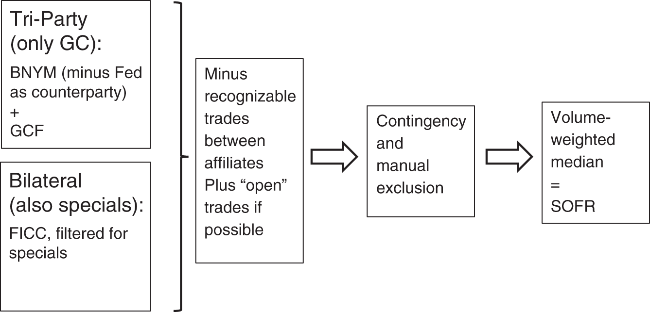
FIGURE 1.2 SOFR: Segments of the repo market used as data input for SOFR calculation
Source: Authors, based on https://www.newyorkfed.org/markets/reference-rates/additional-information-about-reference-rates#information_about_treasury_repo_reference:rates and Federal Register Vol. 82, No. 167
| Page: | https://www.newyorkfed.org/markets/reference-rates/sofr |
| Time: | Approximately 8 a.m. ET for the previous business day |
| Revisions: | Approximately 2:30 p.m. ET for the previous business day
Revisions are possible if additional data became available or an error has been detected and the revised rate differs from the initial one by at least 1 bp. |
| Scope: | 1st, 25th, 50th, 75th and 99th volume-weighted percentiles (50th percentile = SOFR)
Volume Note: The individual repo transactions are not published |
FIGURE 1.3 SOFR: Publication
Source: Authors, based on https://www.newyorkfed.org/markets/reference-rates/sofr
Since liquidity in the repo market is greatest for overnight transactions and decreases rather quickly as the term increases, only the overnight repo market provides the depth required for a reliable reference rate. Hence, the decision to switch from LIBOR to a repo-based reference rate necessitates switching to an overnight term rather than a one-month term or a three-month term, as was the case for LIBOR. This is a key challenge in the transition from LIBOR to SOFR, which will be discussed in Chapter 3.
CALCULATING A REFERENCE REPO RATE
The first task in constructing a reference rate from the repo market consists in collecting data:
- For the bilateral repo market, only data from trades cleared through the delivery-versus-payment (DVP) service of the Fixed Income Clearing Corporation (FICC) is practically accessible.
- For the tri-party repo market, data can be more easily and completely collected from third parties: the FICC offering General Collateral Financing (GCF) repo for its members; and Bank of New York Mellon, acting as clearinghouse. While the former anonymizes brokers, the latter collects data about the counterparties, which can be used to identify repo transactions between affiliates.
The Fed has agreements in place to collect these data from Bank of New York Mellon and from DTCC Solutions LLC, affiliated with FICC. At roughly 8 a.m. the next morning, the New York Fed publishes the volume-weighted median repo rate, rounded to the nearest basis point, as the daily secured overnight financing rate. On publication day only, the Fed will amend this reported SOFR value, in the event it subsequently receives amended data.
The NY Fed does not share the underlying data with the public, the consequences of which will be considered below.
ORIGIN OF REPO RATES USED FOR SOFR CALCULATION
The Fed publishes the volume figures for data used to calculate SOFR, as well as for the Tri-Party General Collateral Rate (TGCR), and the Broad General Collateral Rate (BGCR). As a result, it is possible to gain some insights into the relative volumes that the different sectors of the repo market contribute to the SOFR calculation. The TGCR volume directly represents the volume of tri-party repo rates provided by Bank of New York Mellon. The difference between BGCR and TGCR volumes represents the volume contributed by GCF Repo. And the difference between SOFR and BGCR volumes represents the volume originating from cleared bilateral repo (in each case after the adjustments described in Figure 1.1, such as filtering for specials).
Repo Market Contributions to the SOFR Calculation
Figure 1.4 shows that the volume contributed from GCF repo has been consistently low compared to the other two data sources. The volume provided by Bank of New York Mellon and from cleared bilateral repo has been roughly the same initially, while the latter has been higher since 2019. This graph also suggests that the bilateral repo market, which is only partly captured in the data in Figure 1.4 (only cleared trades, filtered for specials), remains the larger sector compared to tri-party repo.
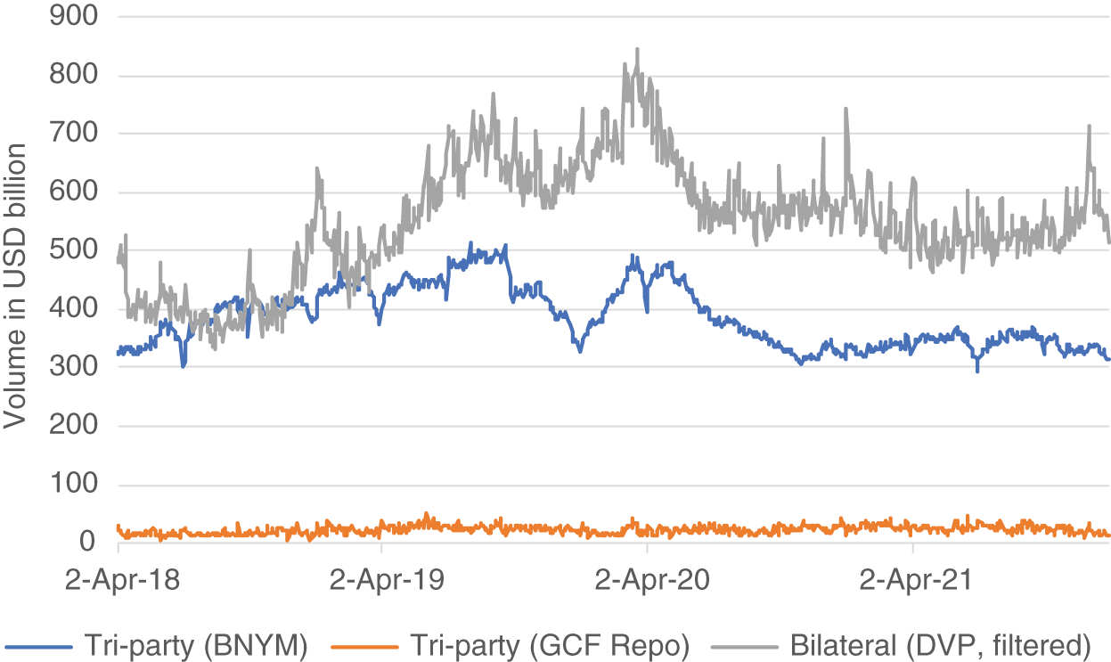
FIGURE 1.4 Volume in different sectors of the repo market
Source: Authors, from data provided by the Fed (https://www.newyorkfed.org/markets/reference-rates/sofr) Disclaimer: These reference rate data are subject to the Terms of Use posted at newyorkfed.org. The New York Fed is not responsible for publication of the reference rate data by the Authors and Wiley does not endorse any particular republication, and has no liability for your use.
Distribution of Repo Rates Used for SOFR Calculation
In addition to the reference rate, defined as the volume-weighted 50th percentile, the Fed also publishes the 1st, 25th, 75th, and 99th percentiles. Figures 1.5 and 1.6 show a history of the rate spreads associated with different percentiles, thereby giving an impression of the width and shape of the distribution. A few observations are worth noting:
- There are significant spikes in the width of the distribution. Most of them coincide with a spike in the level of repo rates (and of SOFR), but not all of them.
- Until the low-interest-rate period starting in April 2020, the distribution tended to be wider on the right-hand side. This may reflect the impact of filtering out most of the special bonds.
- After April 2020, the spikes subsided, and the distribution has exhibited a more symmetric and narrow shape.
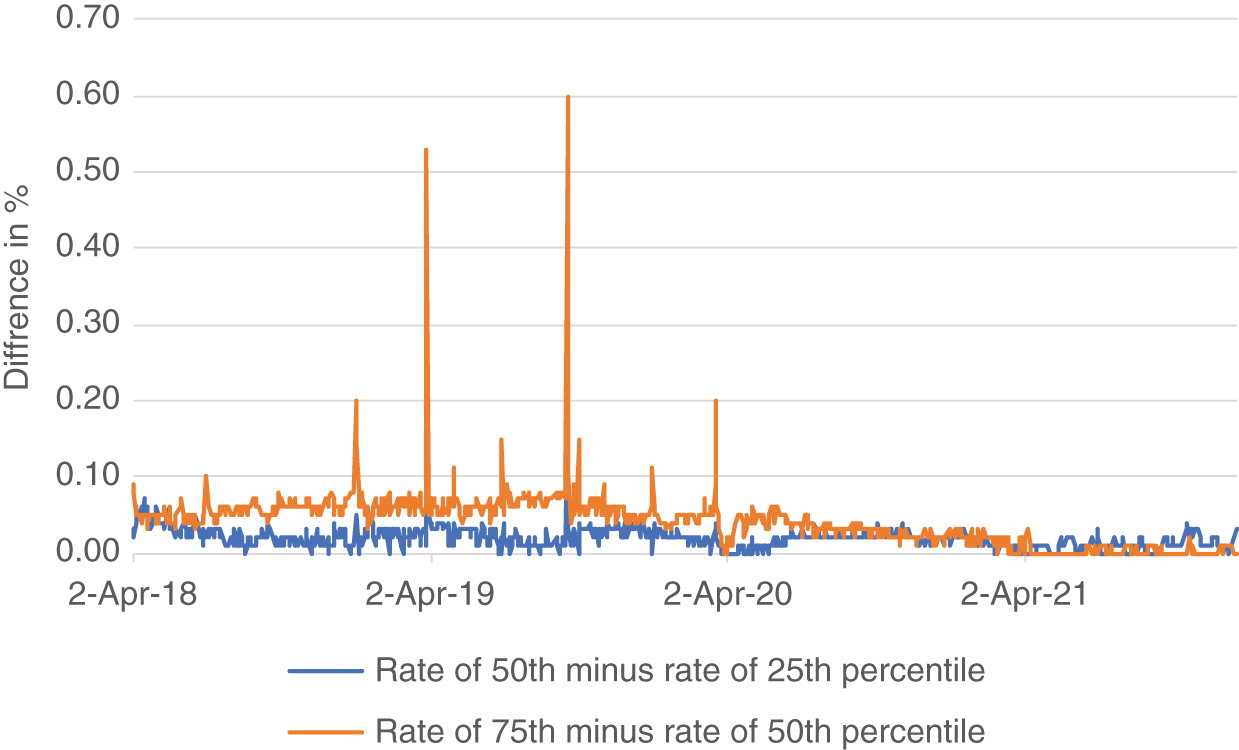
FIGURE 1.5 Difference of rates associated with percentiles
Source: Authors, from data provided by CME
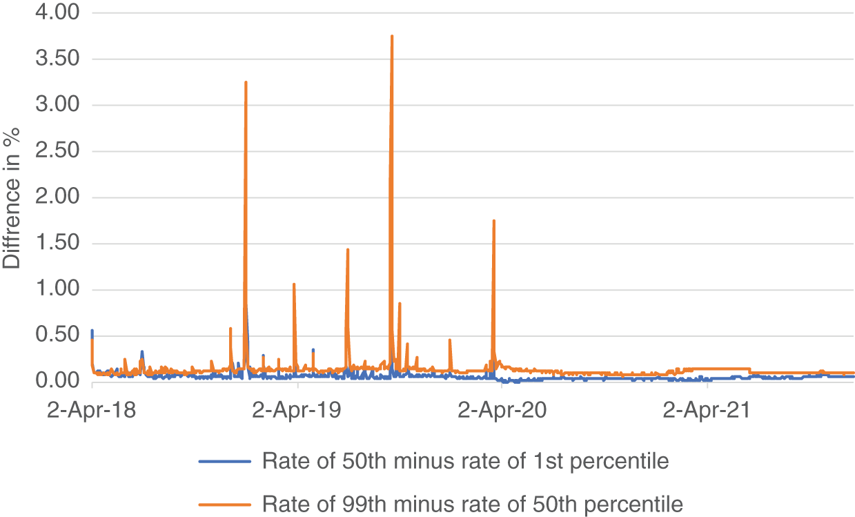
FIGURE 1.6 Difference of rates associated with percentiles
Source: Authors, from data provided by CME
The data filtering applied in SOFR therefore seems to exclude a significant part of the specialness, which results in a relatively narrow distribution on the left-hand side. On the other hand, there is no filtering applied on the right-hand side of the distribution, which means that excessively high repo rates also enter the SOFR data pool, even if they are caused by counterparty-specific factors, such as the difficulty of a bank in accessing funding. On one hand, if funding problems are sufficient to affect the volume-weighted median, they cause a spike in the width of the distribution and the SOFR rate. On the other hand, if funding problems are limited to a smaller subset of banks, they cause a spike only in the width of the distribution. This explains the first observation.
In summary, the data pool for SOFR excludes most bond-specific influences (e.g., specialness) but not the counterparty-specific influences. In other words, the construction of SOFR tends to successfully exclude from the reference rate any instability caused by specialness but not by funding problems. The result is a distribution tilted toward the right-hand side and reflecting general funding stress in a spike of the SOFR rate and of the distribution.
Based on the recent symmetric shape of the distribution, we have calibrated a normal distribution to the percentiles. Specifically, we have calculated the mean and standard deviation of the normal distribution, so that the sum of the absolute differences of its 1st, 25th, 50th, 75th, and 99th percentiles versus those of the SOFR rate becomes minimal. Repeating this calculation for every day, we have obtained the history shown in Figure 1.7.
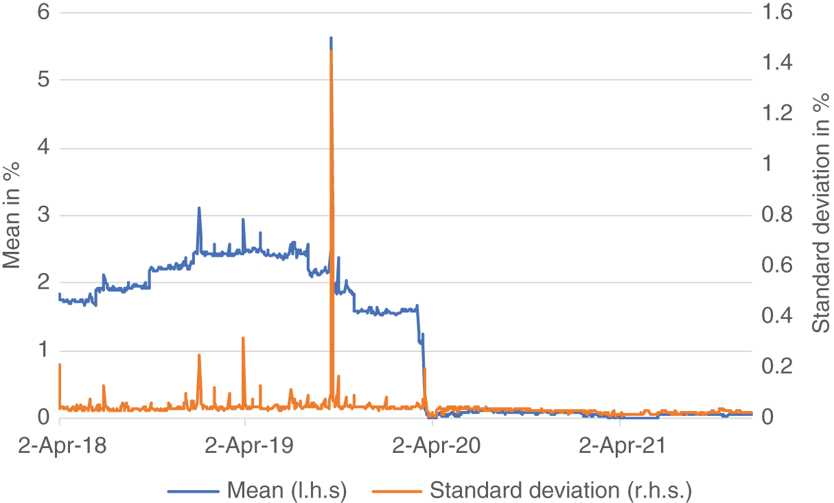
FIGURE 1.7 Mean and standard deviation of a normal distribution fitted to the percentiles of the SOFR data pool
Source: Authors, from data provided by CME
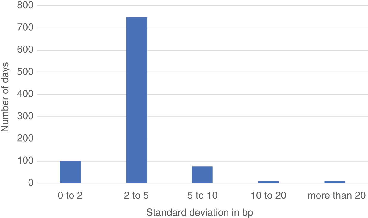
FIGURE 1.8 Histogram of observed standard deviations
Source: Authors, from data provided by CME
As the data of the repo transactions used for SOFR calculation are not published, the distribution obtained in such a manner from the published percentiles can serve as an (imperfect) substitute for further analysis of the repo market underlying SOFR. For example, one can create a histogram of the standard deviation as depicted in Figure 1.8.
On average, the individual repo transactions have exhibited a standard deviation of 4 bp; a standard deviation of more than 10 bp is exceptional.
Repo traders using SOFR (futures) as a hedge should keep in mind this non-negligible standard deviation as well as its sources. In the histogram shown in Figure 1.8, the lower standard deviations tended to occur more recently, so in the current market environment the mismatch between individual repo transactions and SOFR appears to be more benign.
SOFR VERSUS FED FUNDS
Figure 1.9 shows the history of SOFR, a secured overnight rate, along with the history of Fed Funds, an unsecured overnight rate. For scaling reasons, Figure 1.10 shows only the last part of this history, when both rates and their volatility were low. Two basic observations can be made:
- There are instances, even some prolonged periods of time, when SOFR is above the effective Fed Funds rate (EFFR).
- There are significant spikes in SOFR, which are less pronounced in EFFR.
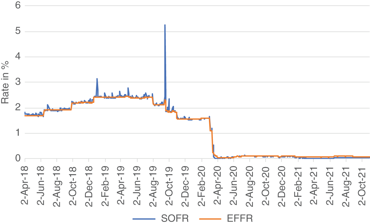
FIGURE 1.9 SOFR versus EFFR
Source: Authors, from data provided by CME
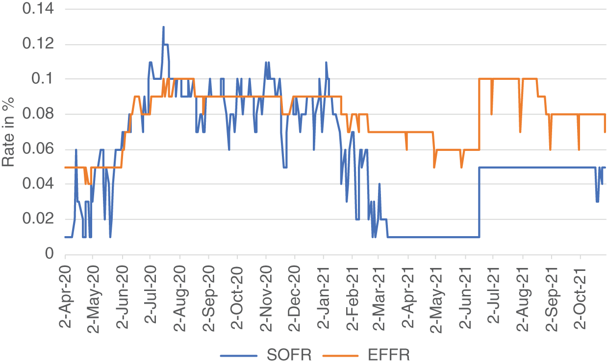
FIGURE 1.10 SOFR versus EFFR
Source: Authors, from data provided by CME
This can be puzzling: Why should a secured rate trade above an unsecured rate for the same tenor? Actually, taking June 29, 2018, as an example, with SOFR at 212 bp and EFFR at 191 bp, a trader could borrow unsecured in the Fed Fund market and lend secured in the repo market overnight, realizing both a profit of 21 bp and a lower risk from collateralization.1 Hence, this transaction fulfills the definition of an arbitrage. Therefore, in efficient markets, SOFR should trade below EFFR. While this has been the case more recently (Figure 1.10), the history of Figure 1.9 tells us that there have been many instances of that arbitrage opportunity, which persisted at times for several weeks.
As a first step to explain the reasons behind this puzzle, we note that participants in secured and unsecured lending markets are partly different. For example, a hedge fund using the bilateral repo market to fund his long positions (and to cover his short positions) in bonds has no access to the Fed Funds market. If hedge funds experience funding problems, the repo rate can therefore rise above the level of Fed Funds (assuming banks using Fed Funds do not experience the same or bigger funding problems). This also explains the counterparty-specific influences on the distribution of repo rates – and why they are usually more pronounced in bilateral repo than in tri-party repo.
Since there exist market participants, such as banks with repo operations, that can participate in both markets and therefore execute the arbitrage, this first step does not solve the puzzle, but only translates it in to the question: Why don't these market participants exploit the arbitrage opportunities whenever they occur?
Following the financial crisis, banks have been subjected to increasing regulation in general and to balance sheet constraints in particular. As a consequence, they need to assess an arbitrage opportunity not only in isolation (as we did in the example of June 29, 2018, above), but also with regard to various balance sheet constraints, such as leverage. When constraints on bank balance sheets are non-binding, banks can execute this arbitrage at relatively low cost. This explains the periods of history when the arbitrage has “worked” as expected and kept SOFR below EFFR. (See Figure 1.10.) On the other hand, when many banks face binding constraints on their balance sheets, increasing the balance sheet via an additional arbitrage position would be costly (e.g., require issuing additional equity). These situations explain the periods of history that exhibited the puzzling observations. Of course, when the arbitrage profit exceeds the cost of executing it, banks are enticed to enter it even when balance sheets are constrained. This explains why the spread remains capped by arbitrage – though the level at which the arbitrage occurs depends on the specific balance sheet situation of banks and can be different from zero.
In summary, therefore, the SOFR–EFFR spread is subject to the arbitrage relationship SOFR ≤ EFFR under the condition that balance sheet constraints allow the bank to execute the arbitrage without additional regulatory costs. The adjustment for regulatory costs will affect the discussion of the basis between secured and unsecured funding rates in Chapter 4.
SOFR SPIKES AND THE SRF
Applying this explanation to the observation of spikes in SOFR, one can see two driving forces:
- A high demand for funding (e.g., during a liquidity crisis) increases both secured and unsecured funding rates.
- A high cost for executing the arbitrage increases secured versus unsecured funding rates.
There is a correlation between both forces. In a general funding crisis, the leverage of banks is usually high, as is the cost of equity required to expand the balance sheet with an arbitrage position. This explains the observation that general spikes in funding rates tend to be more pronounced in SOFR than in EFFR. Imagine a situation of general stress in the financial system, causing hedge funds to push up repo rates versus Fed Funds. A bank may see an arbitrage opportunity but also that its execution would require a costly expansion of its balance sheet at the worst point in time. Hence, the bank will wait for the arbitrage to become large enough to cover the exceptionally high regulatory costs of executing it. A high cost of altering the balance sheet thereby translates directly into the high spikes of SOFR versus EFFR.
Realizing this problem, the Fed decided to assume that role. Specifically, as reaction to the spikes of SOFR, the Fed announced on July 28, 2021, the implementation of a standing repo facility (SRF), providing liquidity to the repo market independently of the balance sheet constraints of banks, with the minimum rate being usually set at the top of the current policy window. In other words, with capital costs becoming too high to make banks a reliable provider of liquidity in repo markets in times of stress, the Fed has introduced, via its repo facility, the SRF rate (SRFR) as an additional constraint,2 i.e.,
The relationship between SOFR and EFFR is therefore determined simultaneously by both of the two constraints, of which the capital cost is unobservable and SRFR is observable. Together this can explain both observations in Figure 1.9, specifically the disappearance of large SOFR spikes once the Fed had introduced the repo facility.
Hence, analysts should keep in mind the structural break in the SOFR time series, which contains both SOFR before and after the Fed repo facility existed (i.e., without and with the SRFR constraint). This situation can be compared to looking at a series of swap rates, to which a cap is added in the middle of the time series. However, due to low interest rates at the point of time the cap was added, this is not immediately visible from the data – but will be once interest rates rise.
While the Fed provides a proxy for SOFR going back far before its introduction (Federal Reserve Bank of New York 2018), it is of limited analytic use, as the SOFR data points were observed in the absence of the constraint. For this book, this leads to the practical problem that at the time of writing (December 2021), there were only a few months of SOFR history available after the introduction of the standing repo facility, which would not have allowed for any meaningful statistical analysis. We therefore needed to ignore the structural break in order to be able to present historical analysis. However, readers should consider this only as an example and repeat the methods presented here once a sufficient history is available with data from August 2021 onward only.
In particular, this has an implication for volatility considerations. (See Chapter 5.) The introduction of the second constraint on SOFR rates also results in a structural break between realized SOFR volatility before and after the point of time of introduction. Consequently, SOFR volatility calculated from time periods before the introduction should be treated with caution. Also, while one could expect some increase in realized SOFR volatility when rates rise, it seems unlikely that the frequency and extent of the spikes visible in Figure 1.9 at higher yield levels will occur again. In fact, from the historical perspective of Figure 1.9, it appears as if the reduction in rates close to zero put an end to SOFR spikes well before the SRF was introduced. However, the existence of the SRF should help mitigate SOFR spikes even in an environment of increasing yield levels. Using the cap analogy from above, the existence of the cap, which is not visible in a low-rate environment, is likely to appear in an environment of higher rates.
As an aside, an Austrian economist would consider the evolution described above as an example of an interventionist cycle (Mises 1924, p. 232). After the state had subjected banks to balance sheet constraints, they became unable to provide repo funding in times of a crisis. This “market failure” gave the state an excuse to “help out” with a repo facility – i.e., to acquire another function that the free market had provided reasonably well before the state intervened.
BENEFITS AND (POTENTIAL) PROBLEMS OF SOFR
Let's finish this chapter by assessing SOFR versus the goals for the new reference rate mentioned at the beginning of this chapter:
- The volume of repo transactions in the data pool for SOFR calculation has been at a consistently high level, as Figure 1.11 demonstrates. While there has been no crisis of the dimension of 2009 since the introduction of SOFR, the pandemic-related crisis did not cause a discernible drop in repo volumes. And repo markets remained functional during 2009 as well. Moreover, the spikes in SOFR do not coincide with significant decreases in volume, meaning that the repo market seems to work well, even during times of general funding stress. These features make SOFR appear favorable in comparison with other reference rates, including LIBOR, which are based on a smaller and/or more unstable transaction volume.
- We have concluded above that SOFR provides a partial solution to the stability goal. It isolates the reference rate from most bond-specific disruptions (e.g., specialness) but not from counterparty-specific disruptions (e.g., funding problems). As a consequence, funding problems affecting a large portion of the financial system cause spikes in SOFR (as in Figure 1.9) and in the width of the distribution (as in Figures 1.5 and 1.6). Funding problems affecting only a small subset (and hence not the volume-weighted median) cause a spike only in the width of the distribution.
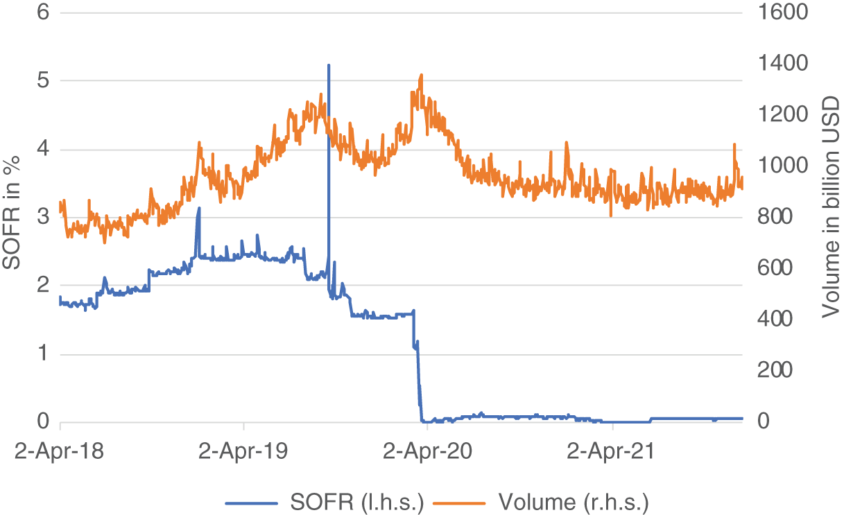
FIGURE 1.11 SOFR rate and volume of repo transactions used for SOFR calculation
Source: Authors, from data provided by CME
The introduction of the Fed's standing repo facility provides an additional part of the solution to the stability goal: It isolates the reference rate also from most counterparty-specific disruptions, such as funding problems.
Taken together, the calculation process excludes most disruptions from the left-hand side of the distribution (e.g., specialness) and from the right-hand side of the distribution (via the SRFR in the equation above).
- So far, SOFR seems to have fulfilled the motivation for its introduction to exclude the possibility of manipulation from the reference rate. However, we see in the construction of SOFR outlined in Figure 1.1 the theoretical loophole of manipulating SOFR via internal repo transactions between affiliates. While these transactions are removed from the Bank of New York Mellon data, where counterparts are visible, this is not possible for the FICC data. On the other hand, given the size of the repo market, the definition of SOFR as the volume-weighted median, and the power of the Fed to exclude doubtful datapoints manually, it appears hard to exploit this theoretical loophole in practice.
It's also worth noting that, while LIBOR calculations are a cross-sectional average, SOFR (like Fed Funds) is a volume-weighted, time-series average. And without access to the volume data, it is impossible for market participants to replicate SOFR via market transactions.
This has two consequences for market participants. First, it's not possible to price SOFR futures purely through no-arbitrage considerations the way we price Treasury bond futures and Eurodollar futures. Anyone trying to trade an arbitrage involving SOFR futures necessarily runs the risk that the published SOFR values that determine the final settlement price of a contract will be different from the repo rate used in the arbitrage. Even for a trader who was active in the repo market throughout the day, it's not possible to replicate the SOFR value with certainty, as the volume information used in the published SOFR calculation is opaque.
The second consequence is that anyone using SOFR futures for general risk management faces this inherent risk every time the contract is used. In most of the examples appearing in this book, we maintain the simplifying assumption that the parties in the example can trade whenever they want at the prevailing SOFR rate. But of course this isn't the case in practice. In practice, market participants are quite likely to be able to trade within a few basis points of the published SOFR value, but there's no way to reduce the residual uncertainty beyond that few basis points. Over time, one would expect the law of large numbers to help, with roughly as many transactions above the reported SOFR value as below. But on any given day, including the day on which the final settlement price of the futures contract is determined, that residual risk remains.
For similar reasons, the decision of the Fed not to share the repo data used for SOFR calculation with the public results in several (potential) problems:
- While some analysis can be done using the percentiles (as above), some important questions remain unanswered. For example, it is impossible to analyze the daily distribution of repo rates and volumes. But this is vital information for a repo dealer quoting an overnight rate in the morning and using SOFR as a hedge. Consequently, obscuring the raw data may result in lesser suitability of SOFR for hedging.
- Likewise, while we have estimated a standard deviation of 4 bp between SOFR and individual repo trades, we needed to assume a normal distribution and calibrate it to the published percentiles. The possibility to conduct analysis on the raw data would lead to better analysis and therefore to better hedges of repo transactions with SOFR and hence to a greater demand for SOFR.
- Big banks with repo desks have access to a part of the raw data in real-time by participating in the repo market determining SOFR, while the general public, including “end users” of SOFR such as smaller banks and corporate borrowers, does not. Consequently, they are in a better position not only to perform some of the analyses mentioned above, but also to estimate the SOFR during the day, before the Fed releases it to the general public on the next business day.
SOFR, TGCR, BGCR, EFFR https://www.newyorkfed.org/markets/reference-rates/sofr SOFR averages and index https://www.newyorkfed.org/markets/reference-rates/sofr Long history of a proxy for SOFR https://www.newyorkfed.org/markets/opolicy/operating_policy_180309 3M SOFR futures https://www.cmegroup.com/markets/interest-rates/stirs/three-month-sofr.quotes.html 1M SOFR futures https://www.cmegroup.com/markets/interest-rates/stirs/one-month-sofr.quotes.html SOFR term rate https://www.cmegroup.com/market-data/cme-group-benchmark-administration/term-sofr.html Source: Authors
- Hence, the secrecy about the raw data may lead to concerns about SOFR being a level playing field. In fact, there seems to be a perception among end users that regulators and big banks have forced SOFR on them, to their potential disadvantage. This perception appears to be the result of several factors, including that the transition from LIBOR to SOFR makes lenders unable to profit from an increase in unsecured versus secured lending rates (see Chapter 4). But sharing the raw data in a timely fashion with the general public would be an essential step for addressing these concerns at their most basic level, by providing more equal knowledge about the reference rate itself. This would enable every participant in SOFR markets at least to see the determinants of its basic reference rate at about the same time and to roughly the same extent.
Overall, the decision not to share the raw data seems to be an “unforced error” in the construction of SOFR, limiting its usability and hence the demand for it, even in its most basic and direct application as a hedge for overnight repo transactions. Fortunately, it can be easily rectified by making its input data publicly available, as the raw data for most other financial transactions and reference rates, such as LIBOR. If the raw data are shared in a timely manner with the general public, the disadvantage of end users versus big banks with repo desks can be mitigated, supporting the acceptance of SOFR as new reference rate.
In case the concern of exposing repo counterparties to squeezes was the reason behind the decision to hide the raw data from the public, anonymizing the counterparties (and maybe also the bonds) could be a solution, which would avoid exploitation of the raw data for squeezes, while at the same time allowing the legitimate analysis described above. Swap Data Repositories might serve as models for publication of the repo data underlying SOFR. A revision of this decision would support the switch from LIBOR to SOFR by allowing smaller end users the same relative degree of transparency enjoyed by banks and other large participants in the repo market.