
CHAPTER 3
SOFR Lending Markets and the Term Rate
As we saw in Chapter 2, the switch from the forward-looking LIBOR term rate to the backward-looking overnight SOFR is relatively easy to implement in the futures market. Both the Eurodollar (ED) futures contract and the SOFR futures contract refer to the same segment of the forward yield curve: ED futures via a forward-looking term rate, and SOFR futures via a backward-looking overnight rate. While the difference between the two has implications for the front-month contract, for back-month contracts the transition from LIBOR to SOFR is almost limited to an exercise in renaming the contract months.
In contrast to the easy implementation in the futures market, the transition to SOFR encounters more resistance in the cash loan market, which would require calculating the interest in arrears if implemented in the same manner as in the futures market. To understand the difficulties involved, consider the example of a borrower, such as a corporate treasurer, used to borrowing at LIBOR term rates. In theory, exactly the same method applied for futures also can be applied to cash loans. Rather than basing lending on forward-looking term rates such as LIBOR, it can be based on backward-looking overnight rates such as SOFR. But for the borrower in our example, this would mean that the rate is determined at the end of the reference period by the SOFR values observed during that period, rather than at the beginning of the loan by a forward-looking LIBOR term rate.
An advantage of applying the transition to backward-looking SOFR reference quarters in both futures and cash loans at the same time and with the same specifications is the ability to use SOFR futures directly as an effective and cost-efficient hedge for cash loans.
In practice, however, mirroring the transition from ED to SOFR futures in the cash loan market has run into several mental, organizational, and technical hurdles:
- Borrowers are used to knowing the interest they need to pay in advance of each period. The corporate treasurer in the example above can report the 3M LIBOR as interest costs to the CEO at the beginning of every lending period; he could therefore be hesitant to embrace the idea of reporting interest costs in arrears based on a reference period of SOFR observations.
- Implementing the same specifications as futures, where cash settlement occurs on the same day that the SOFR value for the last day of the reference quarter is published, would mean that the borrower only learns the size of his next interest payment on the same day he needs to make the payment. This is considered too tight a schedule by many borrowers.
- In addition, relics like simple averaging rather than compounding seem to stick around in some minds and systems, and more so in cash than in derivative markets.
This chapter first outlines these hurdles and possible solutions in greater detail before describing features introduced by the Fed, the ARRC, and the CME with the intention of supporting the cash market transition to SOFR. This concept of “supporting features” comprises
- Model documents and fallback language by the ARRC.
- The publication of simple averages and an index using daily compounding for SOFR by the Fed.
- Using simple averaging for the 1M SOFR contracts at the CME.
- The calculation of a SOFR term rate by the CME.
Overall, it appears that the resolve of regulators to rid the market of the real or perceived market failure inherent in LIBOR met with some resistance in the cash loan market, which led to the provision of several supporting features and compromises.
The biggest compromise from the viewpoint of regulators is the SOFR Term Rate, managed by CME Group Benchmark Administration, which replicates the forward-looking aspects of LIBOR without replicating the LIBOR panel survey process. However, the replacement of the panel survey with a model algorithm results in a different set of issues, as discussed below.
After describing how the tension between the resolve of regulators to switch from LIBOR to SOFR as reference rate on one side and the reluctance of loan market participants on the other side led to the compromise of a SOFR Term Rate, the chapter ends by analyzing two possible scenarios for the further evolution of this construct:
- In the first scenario, the loan market eventually moves closer to the ideal loan mentioned above – a simple SOFR in arrears loan. We characterize this scenario as being “ideal” because the cost of hedging a SOFR loan would be lower in this case and because the structure is preferred by regulators. We expect that the lower costs of hedging this structure will provide an incentive for the loan market eventually to embrace the concept of a backward-looking reference period, in which case a forward-looking term rate may become superfluous.
- In the second scenario, we assume that the reliance on an SOFR term rate will become a permanent feature of SOFR-based lending. In this case, the problem of high hedging costs could be resolved via a secondary market for derivatives based on SOFR term rates – currently discouraged by regulators. Our analysis suggests that the absence of an active derivatives market involving SOFR term rates will likely lead to market imbalances (e.g., involving arbitrage opportunities between term rates and SOFR futures). In the event such imbalances become too disruptive, regulators may be forced to allow interdealer trading of SOFR term rate derivatives. In this scenario, the tension between market desire for a term rate and the regulator's caution may be resolved by regulators giving up on an “ideal” implementation of the transition and accepting the term rate as a permanent feature supported by a secondary market.
This chapter is also the basis for later use cases that analyze the application of SOFR futures and options to hedging cash loans. The further the loan market deviates from the conventions of SOFR futures, the more complex and costlier the hedge.
CONVENTIONS OF SOFR-BASED LENDING MARKETS
The most straightforward loan to hedge with 3M SOFR futures contract is one in which the interest is calculated with daily compounding and paid in arrears – i.e., at the end of the interest reference period. In fact, if the interest reference periods of the loan match the reference periods of the 3M SOFR futures contracts, a near-perfect hedge can be constructed cheaply and easily.1 Similarly, the most straightforward loan to hedge with 1M SOFR futures contracts is one in which the interest is calculated as a simple arithmetic average and paid in arrears.
While these basic loans are straightforward to hedge, they may present problems for other reasons. For example, some borrowers appreciate knowing the size of their next interest payment well in advance of the day they need to make this next interest payment, which isn't the case in these simple loan structures. Given this situation, one can think of solutions, which can be classified by the issue they address:
- The solutions in the first class maintain averaging (arithmetic or geometric) to calculate the size of the next interest payment, but they adjust the date on which the interest payment needs to be made.
- The solutions in the second class allow determination of the interest at the beginning of the interest reference period rather than having to wait until the end of the interest reference period.
While solutions in this first class are designed to help the loan market with the transition to an overnight reference rate, the solutions in the second class can be considered as conceptual capitulations to the concerns of loan market participants. Rather than officials forcing the cash market to switch to interest calculations in arrears, the persistent demand for a term rate forces officials to provide a term rate, which can be used to calculate interest payments in advance.
The first category contains different ways to achieve a longer notification period by introducing a lookback, lockout, or payment delay. We summarize these technical features in Table 3.1 and refer to the comprehensive discussion in The Alternative Reference Rate Committee (ARRC 2021),2 which also contains model language for loan contracts. However, we note that each of these solutions faces new problems. In particular, the longer the lookback or lockout periods, the greater the divergence between the loan and the SOFR futures contracts – and hence the higher the costs and mismatches in a hedge. Chapter 7 will provide use cases illustrating this point.
TABLE 3.1 Conventions for loans in-arrears until (day) T
Source: Authors
| Payment due on day | Use SOFR from day … as SOFR for day d | |
|---|---|---|
| Plain | T+1 | d (for whole period) |
| Lookback (n days) | T+1 | d − n (for whole period) |
| Lockout (n days) | T+1 | d until T − n, then T − n |
| Payment delay (n days) | T+1+n | d (for whole period) |
Given these difficulties, officials have permitted two solutions in which the interest rate is known in advance of the interest reference period:
- From historical SOFR data, i.e., from a period before the lending period. For example, the counterparties could agree to base the interest for a loan during the second quarter on the average of SOFR values observed during the first quarter. While this is technically easy (one simply needs to look up the history of SOFR values3), it introduces the economic mismatch between the two periods. For most participants in the lending markets, this mismatch is unacceptable. In the current situation of low rates, which are expected to increase in coming quarters, this would mean that the borrower is able to pay an outdatedly low interest rate, based on Fed policy of the previous quarter.
- From forward SOFR values, i.e., from market expectations about SOFR values during the lending period. This solves the economic mismatch and the resulting problems of the example above: The lending rate for the next quarter is based on market expectations about Fed policy during that same quarter. And fortunately, as market prices for consecutive 3M forward sectors of the SOFR curve, the SOFR futures provide a good source for these market expectations.4
This overview explains how the tension5 between the regulatory goal of moving from LIBOR to SOFR as reference rate and the practical hurdles of implementing this transition in cash loan markets produced two outcomes:
- Features supporting the technical transition, such as providing model language for lookbacks.
- The introduction of a SOFR term rate, allowing the cash loan market to stick to the “in-advance” structure of LIBOR-based lending (without economic mismatch between periods).
After an overview of the current status of SOFR-based lending markets, we'll discuss these supporting features and term rates in more detail.
STATUS OF SOFR-BASED LENDING MARKETS
As a consequence of the recentness of the switch to SOFR as reference rate, SOFR-based lending markets are still under construction, with a number of conventions being used in parallel. While it is likely that the loan market will eventually settle on a set of standard conventions, at the time of writing (December 2021) it is unclear what this set will be. At the end of this chapter, we will present two scenarios for the future evolution of loan market conventions.
In addition to both in-advance rates and in-arrears rates being used, simple averaging and daily compounding are also currently used in parallel. This introduces an additional dimension to the classification of the SOFR-based lending market. A loan can be in advance or in arrears, and it can use simple averaging or daily compounding. The first dimension classifies loans according to when the interest is determined, the second according to how it is determined. For example, the counterparties may decide to use in arrears with a two-day lookback, i.e., to calculate the interest at the end of the loan period, and then take another independent decision how to calculate the interest, by simple averaging or daily compounding the SOFR observed during the lending period. Based on the choice in that second dimension and the lending period, the ideal hedging instrument may be 1M SOFR futures using simple averaging, or 3M SOFR futures using daily compounding.
And for both choices in the second dimension, supporting features have been introduced:
- The Fed publishes simple averages for standard loan periods of 30, 90, and 180 days.6
- The Fed also publishes an SOFR index implementing compounding, as explained below in more detail.
Under this classification in two dimensions, one can attempt to assess the current status of SOFR lending markets. Both the numbers and statements from market participants underline the importance of the introduction of term rates for activity in SOFR-based lending. Before term rates were introduced, market participants were hesitant to engage in SOFR-based loans; with the advent of SOFR term rates, the transition gained pace. Actually, for most market participants the transition appears to have started with SOFR term rates. This has resulted in in-advance loans using the SOFR term rate currently dominating the market for loans.
Regarding securities based on SOFR such as FRNs, the CME publishes the overall volume of SOFR issuance by tenor and date of issuance7 (Figure 3.1). One can observe a trend toward increasingly issuing longer tenors as well.
Following the recommended model language provided by the Alternative Reference Rate Committee (ARRC 2019), FRNs tend not to use the term rate but an in-arrears interest calculation method. The differentiation between in-advance and in-arrears in the first dimension therefore also captures the overall current status between loans and securities using SOFR.
Regarding the second dimension of this classification, the first securities based on SOFR typically used simple averaging – for example, the first SOFR FRNs issued by agencies. Following the introduction of the SOFR index, however, there seems to be a tendency to use it, and hence the daily compounding embedded in it, for more recent SOFR FRNs.
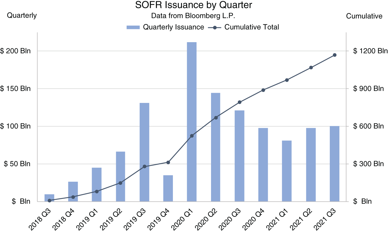
FIGURE 3.1 SOFR issuance by quarter
Source: CME
There is a discussion about the US Treasury issuing a SOFR FRN. This would support the transition by giving the market a benchmark and increasing liquidity. It would also set the standard for conventions; as it appears likely that it will also use the SOFR index, there is a good chance that it will collapse the second dimension for SOFR FRNs to daily compounding only.
SIMPLE AVERAGING VERSUS DAILY COMPOUNDING
Faced with the task of calculating a term rate from a series of known overnight rates, the economically correct approach is to use compounding. With Act/360 as daycount convention, the (ISDA) formula for the term rate R is
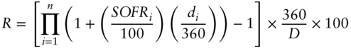
where
- n is the number of business days during the term.
- SOFRi is the SOFR for day i.
- di is the number of calendar days, for which SOFRi is used.
Until the next business day, the SOFR for the previous business day is used, e.g., on weekends and holidays. Thus, if Friday and Monday are business days, the SOFR for Friday is used for Friday, Saturday, and Sunday and the corresponding di is 3.
- D is the total number of calendar days during the term, i.e.,
 .
.
This formula is used both for calculation of the 3M SOFR future settlement price8 (where the term is the reference quarter), in the sample documents provided by ARRC (2019), in the SOFR index (Federal Reserve Bank of New York 2022), and for CME's SOFR term rate, described below (CME October 2021).
In the Excel sheet accompanying this chapter, this formula is applied for calculating the term rate for a one-year loan (from 3 Jan 2022 to 3 Jan 2023). The user can change the level of SOFR for all days or for individual days only and observe the effect. Table 3.2 summarizes the term rate for this loan for different levels of SOFR, assumed to remain constant throughout the year. Of course, rising rates result in a higher spread between the compound term rate and the simple average, which in this case is equal to the constant SOFR listed in the left column.
Simple averaging is still widely used, presumably due to its easier implementation in systems – though the formula above contains no mathematical challenge and can be easily encoded, as the Excel sheet demonstrates. While in the current yield environment the difference between simple averaging and daily compounding may be negligible, it becomes substantial for higher rates, as shown in Table 3.2. This will be an incentive to invest into upgrading the systems to daily compounding. We therefore anticipate increasing yields to be accompanied by an increasing share of daily compounding in the SOFR loan market.
However, as of now, simple averaging seems to be a relic sticking in many minds and systems. Accordingly, the first FRNs based on SOFR issued by agencies used this method. Also, while the 3M SOFR future uses the compounding formula from above, the 1M SOFR future is settled to a simple average. Given that the SOFR futures are leading the development of the SOFR lending market in many ways (as witnessed by the alignment of the conventions recommended by ARRC (2021) with the futures conventions), it appears that a chance has been missed to decide the question in favor of daily compounding for good. Rather than leading the market to use daily compounding by also applying this method to 1M contracts, the 1M and 3M SOFR futures conversely reflect the hesitance of the SOFR market to finally switch to daily compounding only. As a result, the spread shown in Table 3.2 is one influencing factor of the 1M–3M SOFR future spread, as discussed in Table 2.1 of Chapter 2.
TABLE 3.2 Compound term rate for a loan from 3 Jan 2022 to 3 Jan 2023
Source: Authors
| Constant SOFR (bp) | Compound term rate (bp) |
|---|---|
| 0 | 0 |
| 100 | 101 |
| 200 | 202 |
| 300 | 305 |
| 400 | 408 |
| 500 | 513 |
THE SOFR INDEX
In order to facilitate compounding calculations, the Fed has introduced a SOFR index with a base value of 1 for 2 April 2018 (when SOFR started) and updated every business day shortly after the SOFR rate, i.e., after 8 a.m. EST, on its website: https://www.newyorkfed.org/markets/reference-rates/sofr-averages-and-index.
This index implements the formula from above and therefore corresponds to the amount that one would have if one had invested one dollar on 2-Apr-18, earning interest each day at the published SOFR value (i.e., with daily compounding). More specifically, the SOFR index is calculated as
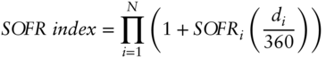
where
- i is the counting number corresponding to a particular business day following 2-Apr-18.
- N is the number of business days since 2-Apr-18.
- SOFRi is the value of the secured overnight financing rate on the ith business day. Unlike CME, the Fed convention is to enter the SOFR value (e.g., 0.015 for a SOFR of 1.5%), hence there is no factor 1/100 in the formula.
- di is the number of calendar days for which SOFRi applies.
The daily SOFR index is rounded to eight decimal places and is subject to revision on publication day only in the same circumstances as those governing revision of the daily SOFR values.
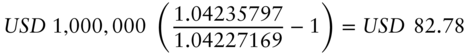
The index is intended to make the use of SOFR products easier for market participants who would rather not have to perform so many calculations themselves. By using this index, the task of calculating the compounded SOFR term rate R simplifies to the equation 9
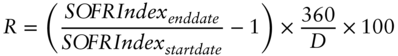
For example, if we wanted to calculate the interest paid on a SOFR-linked loan from 15-Sep-21 to 15-Dec-21, assuming a principal amount of one million dollars, we would divide the SOFR index value for 15-Dec-21 by the SOFR index value for 15-Sep-21, subtract 1, and then multiply the result by one million. In this case the interest payment would be
TERM RATE
We have attempted to explain above how the tension between the regulatory drive to switch from LIBOR to SOFR as reference rate on one side and the resistance of loan market participants on the other side has resulted in the compromise of introducing a term rate for SOFR, allowing the replication of LIBOR conventions. As with the forward-looking term rate LIBOR, a borrower can then use a forward-looking SOFR term rate and stick to the “in advance” specifications he is used to.
At this point of the evolving discussion, the question became how to determine the SOFR term rate. Reading through the following list of possibilities made the decision easy:
- The term rate could be set by administrative or expert judgment. However, this would introduce a potential friction between lending markets based on a term rate set this way and the actual SOFR markets.
- The term rate could be obtained via a survey of market participants about their perception of the current market for SOFR forward rates. For instance, one could call a number of contributor panel banks at 11 a.m. This option is obviously the nightmare of regulators as it would counteract the fundamental goal behind the whole SOFR project. Fortunately, as there exists an SOFR futures market, a survey is not needed to assess the market for forward SOFR. This decided in favor of the last option:
- A term rate could be calculated from the prices of SOFR futures contracts – being market prices for consecutive 1M and 3M parts of forward SOFR – via an automatic model without any expert judgment.
Hence, the existence of an active SOFR future market makes it possible to translate the market prices for forward SOFR into SOFR term rates without the interference of an administrator or a panel via the use of an automated model – which has its own set of potential problems, as discussed below. But given the alternatives, it seems to be the best way to translate an actual market for forward SOFR into an SOFR term rate. The SOFR term rate calculated this way allows loan market participants to calculate interest in advance while achieving the goal of regulators not to replicate LIBOR's method of determining term rates via a survey. This compromise was therefore the endpoint of the tension and discussion described above (ARRC 2021, p. 25).
To our knowledge, this is the first instance where term rates have entered a market via and after futures. The path of this construction is reflected in the sequence of chapters of this book: Overnight SOFR (Chapter 1) ➔ SOFR futures (Chapter 2) ➔ SOFR term rates (Chapter 3).
THE MODEL TRANSLATING SOFR FUTURE PRICES IN SOFR TERM RATES
The CME has implemented the model outlined by Heitfield and Park (2019) to extract 1M, 3M, 6M, and 12M Term Rates from SOFR futures. The details of this process have been published (CME October 2021). Summarizing the key aspects in Figures 3.2 and 3.3, in a first step, the data from future markets are aggregated by using sampling techniques and observation intervals in order to minimize effects from outliers and periods of illiquidity. While currently only data from the future markets are used, SOFR OIS (Overnight Index Swaps) may be considered as an addition in future.
At the core of the model is a jump process, which is then fitted to the aggregated data.10 This process assumes that SOFR can change only after FOMC policy rate announcements and remains constant otherwise. That is a pretty strong assumption, which could affect the term rates calculated via this model, as discussed below. In more detail, an optimization algorithm fits the following process for SOFR to the observed data:
where
- t0 is the start of the term.
- M is the set of all FOMC policy announcement dates between t0 and t.
- jk is the jump of SOFR following the FOMC policy announcement on day k.
CME term rates are then obtained by compounding the daily SOFR of this jump process using the ISDA formula from above.
CRITICISM OF THE CME TERM RATE
The CME Term Rate calculated via this approach can be criticized on two levels: in general, that a model is used at all for determining term rates; and specifically, which model is used. The published SOFR term rates reflect the future market as seen through a specific model and its assumptions. At the end of Chapter 2 (Table 2.2), we have demonstrated the significant effect of process and parameter selection on the pricing. And the assumptions of using a pure jump process are quite strong, e.g., they imply that neither mean reversion (other than captured in the jumps) nor momentum nor volatility unrelated to Fed policy has an effect on SOFR values, with a correspondingly high probability of distorting the information from future markets.
Given the list of alternatives above, it seems quite likely that determining term rates via a model (rather than by expert judgment or a market survey) from the market prices for forward SOFR values observable in the future markets is the best among the available options. However, since using a model introduces its own specific problem of distorting the observed market by the model assumptions (rather than by expert judgment or a market survey), care should be taken when selecting the model in order to minimize the distortion. And from the documents available to the public, it does not seem that much discussion took place about the model selection. In fact, it appears that the approach of Heitfield and Park (2019) has been implemented without investigating less-restrictive alternatives:
| Terms | 1M, 3M, 6M, 12M |
|---|---|
| Publication | At 5 a.m. CT on every day SOFR is published |
| Start of term | Second business day (included) after publication day |
| Data input | Future market of the business day preceding publication day |
| The first 13 1M SOFR contracts and the first 5 3M SOFR contracts are used | |
| (those during their reference quarter are adjusted for the known rates) | |
| Observation Intervals | 14 periods of 30 min from 7 a.m. to 2 p.m. CT |
| Sampling | VWAP (Volume Weighted Average Price) of executed transactions from DCM (1) and a snapshot of executable bids and offers at a random time during the interval (2) |
| Aggregation | An observation interval is eligible, if it contains an executed transaction in any SOFR future |
| |
| |
| |
| Future price used as input in the model is calculated as VWAP over all eligible observation periods of the day | |
| (if there is no interval with an execution, the previous day's price will be used) |
FIGURE 3.2 SOFR term rates: specifications
Source: Authors, based on CME
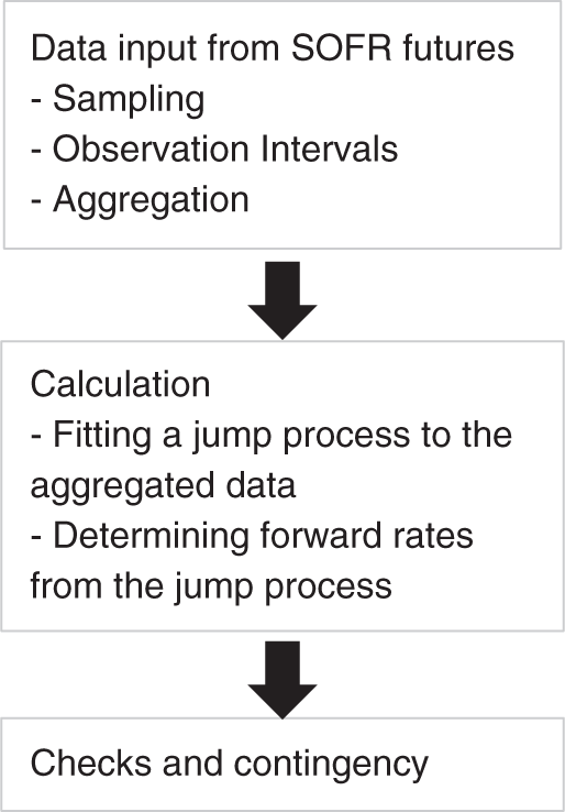
FIGURE 3.3 SOFR term rates: calculation process
Source: Authors, based on CME
- By construction, the jump process used allows changes of the interest rate only after FOMC policy announcements and hence ignores all other factors influencing SOFR values and all rate volatility between meetings. In light of the SOFR spikes (Figure 1.9) that appears to be a strong assumption imposed on the market, which puts the term rates calculated under this assumption at a significant risk of distorting the market information. While the introduction of the Fed's standing repo facility (SRF) may well bring the market somewhat closer to this assumption (see the additional constraint SOFR ≤ SRFR mentioned in Chapter 1), it is not sufficient to conclude that non-policy-related volatility will be absent from the repo market. This deficiency could be addressed by using a mixed jump-diffusion process.
- Moreover, the volatility not coming from Fed policy has a significant effect on the prices of options on SOFR futures. (See Chapter 5 and Table 5.2 in particular.) Hence, the pure jump process used to calculate the term rate cannot be used to obtain reasonable option prices. And using two different models opens the door for inconsistencies between both.
- There are alternative ways to achieve the extraction of constant-maturity term rates from curves, which have been proven to work well in other markets but which do not seem to have been considered for SOFR term rates. For instance, spline models – available in different forms11 – tend to do a good job for obtaining constant maturity par (or zero) yields from bond markets. In the spline model we presented in Chapter 11 of Huggins and Schaller (2013), the Fed meetings could be easily incorporated as external variables. This would allow accounting for their effect as external shocks while preserving the internal dynamics and volatility of rates.
- Even if one accepts the process in general, one can still argue about its implementation. For instance, the optimization implemented by the CME results in the Term Rates being influenced by futures beyond the end date of the term. The 3M Term Rate could depend partly on futures whose reference periods start in 6M time, for example. By contrast, the term rate hedge described in Chapter 2 only uses futures, whose references periods coincide with the term. Market participants usually prefer this feature, since it is unintuitive that a term rate should depend on events such as FOMC meetings taking place after the horizon of the term.
Hence, while criticism on the general level about using a model at all can be countered by the lack of better alternatives, criticism on the specific level about the model selected for calculating the term rate appears to be valid. Researching other models with the goal of minimizing the impact of the model assumptions on the translation of future prices into term rates and depending on the results replacing the basic jump process in the CME's Term Rate model would be the best way to counter this specific criticism.
In addition, some participants have expressed concern about the limited liquidity of SOFR futures (i.e., of the data basis for the term rate calculation) (see, e.g., Bowman n.d.). In terms of Figure 3.3, this criticism focuses on the first step, the criticism of the model on the second. However, taking into account the sampling techniques and observation intervals mentioned above and the expected further increase of liquidity following the migration from ED contracts, the concern about liquidity seems to be both sufficiently addressed and of a temporary nature. A general adoption of compounding would also help by concentrating liquidity in 3M contracts.12
Chapter 8 will describe a precise hedge of the CME's Term Rate with CME SOFR futures and shed additional light on this discussion from the perspective of the practical hedger.
TWO SCENARIOS FOR THE FURTHER EVOLUTION OF THE TENSION AND HENCE THE TERM RATE
We have described the CME Term Rate as the product of a compromise between the goal of regulators to move the lending market away from LIBOR to SOFR and the demands of loan market participants and have seen that the introduction of this compromise product has been key to achieving acceptance of and activity in SOFR-based lending markets.
However, this compromise does not resolve the underlying tension but rather embodies it. It seems likely, therefore, that the tension will continue until it is resolved one way or another. In the following, we will present two scenarios for the further evolution of this tension and consider the effect on its current compromise product, the CME SOFR Term Rate.
Scenario 1: Shift Away from the Term Rate Due to High Hedging Costs
As we've seen, hedging a SOFR loan with the rate calculated and paid in arrears is a straightforward process, as SOFR futures can be used directly (1M futures when the loan rate is calculated via a simple average and 3M futures when the loan rate is calculated using daily compounding). By contrast, hedging CME's term rate requires replicating the rather complex data aggregation and calculation described in Chapter 8. In the end, the loan using a term rate is also hedged with SOFR futures – but via expensive replication (or by paying a premium to a dealer for taking the risk of imperfect replication). Currently, the cost of hedging the term rate is multiple basis points (E. Childs, personal communication), i.e., one order of magnitude greater than the cost of hedging directly with futures.
From an economic perspective, using term rates therefore seems to be a costly way to the same outcome – hedging with SOFR futures (ARRC 2021, p. 28).13 Thus, the ability to achieve the same hedge in a much cheaper and more direct way should be a major incentive for borrowers to embrace loan structures that are very similar to the specifications of the CME SOFR futures contracts. While the costs of adjusting systems may vary between different companies, the more and the larger hedges are executed, the earlier this investment will pay off. The significant difference between direct and indirect hedging costs suggests that this breakeven could be reached rather soon except perhaps for the least active and smallest borrowers.
The more the lending market develops according to this forecast – that is, the closer it resembles the ideal situation described at the beginning – the less the supporting features will be required:
- The demand for the term rate, which allows for in-advance SOFR lending, depends on the resistance to move toward in-arrears, i.e., in the first dimension of the transition.
- The demand for simple averaging and related products (like 1M SOFR futures) depends on the resistance to move toward compounding (i.e., in the second dimension of the transition).
In other words, the more complete the transition of the lending market to SOFR will be, the more ephemeral the Term Rate and products using simple conventions are likely to be.
In this scenario, the “ideal” hedgeability of in-arrears loans supports via lower hedging costs the “ideal” envisioned by regulators. The current compromise product of a SOFR Term Rate could then be an ephemeral phenomenon only, which will disappear together with the reluctance of the cash loan market. The tension is solved by one part of it receding and its current product of a term rate will disappear with it.
At the core of this issue is the statement of the general model critique above: that Term Rates represent the future markets as seen through the model and its assumptions. This results in the hedging problem that (unlike loans using in-arrears) the term rate cannot be directly and cheaply hedged with futures, but only indirectly and expensively via an additional replication of the model and its assumptions. Chapter 8 will demonstrate how to do this and thereby give an impression of the complexity involved in hedging CME's Term Rate.
Scenario 2: Persistence of the Term Rate and Consequences
The hedging costs of term rates could be reduced via an active secondary market for term rates, allowing dealers to pass on term rate exposure rather than charging a high premium for either taking over that exposure or going through the complex exercise of replicating the model. However, regulators are prohibiting a secondary market: Banks are allowed to deal the term rate with “end users” only – for example, to hedge a loan based on the SOFR term rate, but not to deal the term rate between themselves.
We suppose that the reason for that prohibition of interdealer trading in the term rate is precisely the motivation to keep hedging costs for loans based on the term rate high and thereby maintain the incentive to move toward in-arrears described in scenario 1 above. While we have not found any official documents explaining the reasons behind the prohibition of a secondary market for the term rate, this appears to be the only possible explanation for US officials interfering in such a severe way with the development of free markets.
In terms of the tension between regulatory goals and market needs, which described the evolution toward the term rate, one can state that this tension is currently embodied in the hedging problem and the high hedging costs of term rates. Via prohibition of a secondary market for term rates, regulators keep this tension and the hedging costs high in order to nudge the loan market toward their preferred scenario 1, which resolves the tension in the hedge by the hedging product disappearing. An alternative solution to the tension currently embodied in high hedging costs for term rate loans would be the development of a secondary market, leading to efficient hedges of the term rate and hence supporting its permanence. Hence, by prohibiting this secondary market, regulators express their continuing disapproval of the term rate by depriving it of a cheap hedge.
Under the assumption of this scenario that the term rate remains as central to SOFR lending as it is now, we can analyze the likely consequences of the prohibition of a secondary market and thereby try to anticipate the possible future issues. Like the evolution of the tension has led to the current situation of lending markets using a term rate, the tension embodied in the term rate will determine their further evolution.
Taking the perspective of a dealer hedging loans based on the SOFR term rate, he cannot unload his risk by using a secondary market for the SOFR term rate, but needs to use other hedging products, specifically SOFR futures, e.g., by trying to replicate the calculation process of the term rate as closely as possible (see above). This introduces a bias into future markets, as all dealers hedging SOFR term rates are on the same side. Currently, the share of term rate hedging in overall SOFR future trading is still small, and such a bias is not visible to us – but this scenario assumes that lending based on the term rate will become the standard. The more loans using the term rate are hedged, the more visible the bias will be. Moreover, an increase of rates and volatility from the current historically low levels is likely to result in increased hedging activity, both of cash loan market participants hedging their SOFR term rate exposure with dealers and of these dealers hedging their SOFR term rate exposure with futures. In terms of our tension concept, this would mean that the tension currently embodied into the term rate (and the prohibition of a secondary market) evolves into a discrepancy between the markets for the SOFR term rate and for SOFR futures.
Thinking further through this scenario, this bias would be an attractive arbitrage opportunity for those who can make use of it, i.e., are not subject to the regulatory prohibition of interdealer trading in the SOFR term rate. For example, foreign banks might be able to execute this arbitrage – by using the CCBS (Cross Currency Basis Swap) to gain access to USD. In this case, their arbitrage may result in removing the bias from SOFR futures – but transform it into a bias in the CCBS market. Using the terms of our concept again, this would mean that the tension evolves into a mispricing in the CCBS market. This would be another arbitrage opportunity, which another group of market participants may be able to exploit, thereby continuing the evolution of the tension through different markets and countries.
Given that the consequences of this scenario, such as mispriced SOFR futures and arbitrage opportunities for foreign banks, are unattractive to regulators, it seems likely that they would reconsider the prohibition of a secondary market for the term rate. Hence, over time the persistence of SOFR term rates could lead to regulators accepting it as a permanent solution and allowing the interdealer trading necessary to support it. In contrast to the first scenario of the tension being finally resolved by the market converging to the “ideal” of regulators, in the second scenario the tension is resolved by regulators giving up their fight against the demand of loan markets for a term rate and accepting its permanence by giving up their fight against a secondary market. It seems unsustainable that banks will build large one-way exposures to SOFR term rates if they can't manage those exposures. It seems more likely that either banks will eventually pull back from offering loans linked to term SOFR rates or that regulators will relent and allow banks to manage these exposures in the OTC derivatives markets.
In a broader perspective, the possible evolution of this tension through the markets (maybe via futures to CCBS) is an example for arbitrage opportunities caused by regulatory intervention.14 As long as demand for the term rate and the prohibition of a secondary market maintain the tension, it is likely to cause mispricings and hence profit for arbitrageurs.
In summary, the final resolution of the tension causing the current high hedging costs for loans using the term rate is achieved:
- In scenario 1 by regulators maintaining this high cost until the hedged product “term rate” disappears and the loan market has moved toward their ideal of in-arrears, which can be directly and cheaply hedged with futures.
- In scenario 2 by regulators finally allowing the secondary market as an alternative hedge for term rate loans, i.e., by the hedging costs for term rates becoming less prohibitive and the loan market achieving the permanence of its preferred alternative through a liquid interdealer market for the term rate.
NOTES
- 1 We characterize the hedge as near-perfect rather than perfect due to the possible effects of any interest paid or received on variation margin.
- 2 See also https://www.newyorkfed.org/medialibrary/microsites/arrc/files/2019/Guide_to_SOFR.pdf.
- 3 For standard loan periods, the Fed even publishes historical averages.
- 4 The predictive quality of forward rates for actual rates (and policy) has been subjected to an extensive and controversial analysis, which we will not repeat here.
- 5 The Alternative Reference Rate Committee (ARRC 2020) and https://www.newyorkfed.org/medialibrary/microsites/arrc/files/2019/Guide_to_SOFR.pdf are good historical documents for this tension and the discussion among officials and market participants.
- 6 Also on the website https://www.newyorkfed.org/markets/reference-rates/sofr.
- 7 See the CME Group website at https://www.cmegroup.com/trading/interest-rates/secured-overnight-financing-rate-futures.html?utm_source=cmegroup&utm_medium=friendly&utm_campaign=sofr&utm_content=sofr&redirect=/sofr#sofrissuance.
- 8 SOFR Futures, “SOFR Futures Settlement Calculation,” 2019, https://www.cmegroup.com/education/files/sofr-futures-settlement-calculation-methodologies.pdf.
- 9 See the Federal Reserve Bank of New York, “Additional Information about Reference Rates Administered by the New York Fed,” January 24, 2022, https://www.newyorkfed.org/markets/reference-rates/additional-information-about-reference-rates#sofr_ai_calculation_methodology.
- 10 Chapter 8 describes the fitting in more detail.
- 11 For the short end of the curve, cubic splines usually produce better results than exponential splines.
- 12 On the other hand, this would introduce a specification difference between 1M SOFR and Fed Fund futures, losing this contract spread as a clean expression of the secured–unsecured basis for the next chapter.
- 13 The Alternative Reference Rate Committee presents a similar argument for hedges with SOFR OIS swaps. We feel that the point becomes even clearer when considering hedges with SOFR futures.
- 14 Chapter 18 of Huggins and Schaller (2013) outlines this process in general.