
![]()
Querying and Analyzing Patterns
There are different ways to step into data visualization, starting with the analytics strategy that should allow us to identify patterns in real time in our data, and also to leverage the already ingested data by using them in continuous processing. This is what we’ll cover in this chapter through the integration of Spark, the analytics in Elasticsearch, and finally visualizing the result of our work in Kibana.
Definining an Analytics Strategy
In this section we’ll go through two different approaches for analyzing our data, whether we want to continuously process our data and update the analytics in our document store or make real-time queries as the demand comes. We will see at the end that there is no black-and-white strategy in a scalable architecture; you will likely end up doing both, but you usually start with one of them.
What I call continuous processing is the ability to extract KPI and metrics from batch of data as they come. This is a common use case in a streaming architecture that once set up can bring a lot of benefits. The idea here is to rely on a technology, which is:
- Distributed
- Resilient
- Does the processing in near real time
- Is scalable in term of server and processing
Spark is a good candidate to play this role in the architecture; you can basically integrate Spark and Kafka to implement continuous batch processing. Indeed, Spark will consume messages from Kafka topics in batch intervals and apply processing to the data before indexing it into a data store, obviously Elasticsearch:
- The first benefit is to save the datastore from doing the processing
- The second one is to be able to have processing layer such as Spark that can scale. You will be able to add more Spark Kafka consumer that does different kind of processing over time.
The typical processing done is an aggregation of the batch data such as, in our example, number of queries, number of 404 errors, volume of data exchange with users over time, and so on. But, eventually, this processing can reach the point where we do prediction, on data by using the machine learning features of Spark.
Once processed data are delivered by Kafka, streamed and processed by Spark, they should be available for analytics and search. This is where Elasticsearch comes into play and will allow the user to access in real time to data.
Real-time querying removes the burden of relying on a tradional batch processing architecture such as a Hadoop-oriented distribution, which can be heavy to deploy and is not what end users expect.
Today, you typically want the information now, not in five minutes or the next day.
The strategy of real-time queryring is efficient depending on the datastore you are dealing with. It should also provide a set of API that let the users extract essential information from a large set of data at scale.
Elasticsearch does tis: it supports running aggregation queries through the aggregation framework to group document or compute document field data in near real time.
With real-time querying and the out-of-the-box aggregation capabilities of Elasticsearch, we can have an ingestion pipeline that gets rid of any processing between the time that the data have been ingested, to the moment the data are indexed in Elasticsearch. In other words, the pipeline can be reduced to draining the data from Kafka with Logstash and indexing them into Elasticsearch.
The idea here is to see what you should do in Spark and what you should keep for Elasticsearch. We’ll see that implementing simple grouping aggregation could be very handy with Elasticsearch.
Process and Index Data Using Spark
To ingest the data with Spark we first need to implement a Spark streaming agent that will consume the data from Kafka and then process and index them in Elasticsearch. Let’s then split the ingestion with Spark into two parts: the streamer and the indexer.
![]() Note that code used in this chapter can be found in the following repo: https://github.com/bahaaldine/scalable-big-data-architecture/tree/master/chapter5/spark-scala-streamer
Note that code used in this chapter can be found in the following repo: https://github.com/bahaaldine/scalable-big-data-architecture/tree/master/chapter5/spark-scala-streamer
Preparing the Spark Project
To implement the streaming agent, we’ll use Spark Streaming, a reliable, fault-tolerant API that is used to stream data from variant data sources. More information can be found at:
https://spark.apache.org/streaming/
So far, we won’t structure the data that we receive. The goal here is to set up the streaming itself, ingest the stream from Kafka, and be able to print it out. I’m used to Eclipse (Mars 4.5) to implement my Java (1.8)/Scala(2.10) project. IntelliJ is also a really good IDE and very popular for Scala applications.
The first thing we need to do is to create a Spark project structure with needed dependencies. To do so, we’ll use Maven and a Spark archetype that you can easily find on Github. In my example, I’ll use:
https://github.com/mbonaci/spark-archetype-scala
We this archetype you can simply generate a Scala project that you can then use in Eclipse Execute the command shown in Listing 5-1.
![]() Note that the escape character used here to break the line should be adapted to the OS; for example, that would be « ^ » on windows.
Note that the escape character used here to break the line should be adapted to the OS; for example, that would be « ^ » on windows.
Maven will prompt and ask for confirmation prior to generating the project. Go through those steps and finalize the creation. You should then have the directory structure like that shown in Figure 5-1.
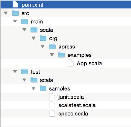
Figure 5-1. Spark Scala project directory structure
This directory structure is really important in order for Maven to be able to compile and package your application correctly.
First thing we are going to do is to understand the sample application that Maven has generated for us.
Understanding a Basic Spark Application
The Spark archetype has the benefit of generating a sample application that gives the basic structure of a Spark program. It first starts with the configuration of the Spark context, then handles the data processing, and sends to an output the result of that processing.
In the sample program (App.scala file), the configuration of the SparkContext consists of setting the Application name that will appear in the cluster metadata and the cluster on which we will execute the application, as shown in Listing 5-2.
We use the special value of local[2] here, which means that we want to run the application on our local machine using a local Spark runtime with two threads. That’s really convenient for testing purposes and we’ll use this method in this book.
Once the configuration is done, we will create a new Spark configuration using the configuration shown in Listing 5-3.
Then the sample program creates a dataset, shown in Listing 5-4.
There are actually two steps in this line of code:
- it first creates a collection holding every five numbers from 0 to 100
- Then Spark parallelizes the collection by copying it into a distributed dataset. In other words, and depending on the topology of the cluster, Spark will operate on this dataset in parallel. This dataset is commonly called a Resilient Distributed Data (RDD.
Note that here we don’t set the number of partitions that we want to split the dataset into because we let Spark take care of this, but we could have partionned our data like that shown in Listing 5-5.
Finally, we transform our data using the Spark sample function, which produces a new RDD containing a new collection of value, as shown in Listing 5-6.
Here we use a number generator seed of four. If you want to print out the content of the generated sample, use a mirror map function like that shown in Listing 5-7.
This will print out something like that shown in Listing 5-8.
If you run the sample application using the Listing 5-9 command:
the last part of the code (Listing 5-10:
will print out:
This Spark application is called a Spark driver. Obviously, this one is really easy to understand and uses a few features, but it gives the general idea of a driver structure. What we want to achieve with Spark in our use case is to be able to process a large amount of data, in a distributed way, and digest them before sending them downstream in the architecture.
Implementing the Spark Streamer
Introducing Spark in our existing architecture doesn’t require to modify what we have seen in Chapter 4; it’s just a matter of adding a new consumer to our Kafka clickstream topic like that shown in Figure 5-2.
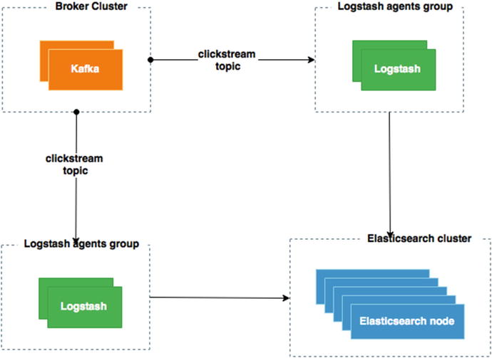
Figure 5-2. Adding Spark Kafka streaming to our architecture
Our Spark driver should be able to connect to Kafka and consume the data stream. To do so, we will configure a special Spark context called Streaming context, as shown in Listing 5-12.
As you can see, the context configuration is pretty much the same as that in the previous sample Spark driver, with the following differences:
- We use the es.index.auto.create option to make sure that the index will be created automatically in Elasticsearch when the data is indexed.
- We set the StreamingContext at a 2-second batch interval, which means that data will be streamed every 2 seconds from the Kafka topic.
We need now to configure from what brokers and what topics we want to receive the data, and then create the stream line between the two worlds, as shown in Listing 5-13.
The args variable contains the arguments passed to the driver when running it. The list of brokers and list of topics are both delimited by a comma. Once parsed, the KafkaUtils class, provided as part of the Spark streaming framework (org.apache.spark.streaming package), is used to create a direct stream between Kafka and Spark. In our example all messages are received in the messages variable.
At this point we should be able to output each streamed clickstream log line by using the map function in Listing 5-14.
There are a couple of things to examine in the previous lines:
- the messages variables is an RDD that holds the streamed data
- the _ syntax represents an argument in an anonymous function, as in Listing 5-15.
This is equivalent to the line shown in Listing 5-16, where _2 is the second element of the x tuple.
To run the driver, we’ll first build it using maven. Run the following command to compile and package the Scala code into a JAR:
mvn scala:compile package
Note that in the case of that driver, I’m using Scala 2.10.5, which requires Java 7 in order to work:
export JAVA_HOME=/Library/Java/JavaVirtualMachines/jdk1.7.0_21.jdk/Contents/Home/
Once compiled and packaged, you should end up with a two JARs in the project target directory:
- spark-scala-streamer-1.0.0.jar: contains only the compiled project classes
- spark-scala-streamer-1.0.0-jar-with-dependencies.jar contains compiled classes and project dependencies
We’ll use a slightly different method than in the previous part to run the driver: the spark-submit executable from the standard spark distribution, which can be downloaded from here:
http://spark.apache.org/downloads.html
At the time of the writing I was using the 1.4.0 version. Once downloaded I recommend that you simply add Spark binaries to your PATH environment variable, as shown in Listing 5-17.
This will ease the access to all Spark executables including spark-submit that you can use like that in Listing 5-18 to execute our previous program.
As you can see, we pass the KafkaStreamer to spark-submit, which is part of the JAR we just created. We are using the JAR with dependencies because otherwise Spark will not find the needed class and you will likely end up with a “class not found” exception. At the end of the command, you have probably recognized the argument containing the broker list that we want to connect to and the topic that we want to stream data from. Running this command just bootstraps Spark and listen for incoming message, thus generate log lines using the generator we used in the previous and be sure that the streaming pipeline is running in order to push message in Kafka. You should get some lines outputted in the console like those in Listing 5-19.
Now that we have the streaming part of our code running, we can focus on the indexing part.
Implementing a Spark Indexer
The indexing part is the last part of our driver but, surprisingly, we are not pushing its configuration to the last step.
What we will do here is just make sure that each clickstream event that we consume can be indexed in ElasticSearch. The clickstream events are actually JSON received in string stream; we then need to parse the string, marshal to JSON RDD, and then create a RDD of Clickstream object.
Let’s first defined our Clickstream object as shown in Listing 5-20.
Except for the bytes, we assume that every field are Strings. Let’s now parse our lines of JSON String as shown in Listing 5-21.
Lines are processed in two steps:
- each lines is parsed using JSON.parseFull
- for each JSON, RDD are transformed into a map of key and value.
Finally, clickstream events RDD are pulled out from the parsedEvents variable as shown in Listing 5-22.
We simply make a mapping between each parsed event Map and new Clickstream event object. Then at the end we index the data using the Elasticsearch Hadoop connector as shown in Listing 5-23.
I’m creating a different index than the one created by Logstash in the previous chapter. The data are in the spark index under the clickstream type.
You can find more information on the Elasticsearch Hadoop connector at this link:
https://www.elastic.co/guide/en/elasticsearch/hadoop/current/index.html
At this point you should be able to index in Elasticsearch after generating data, like in Figure 5-3.
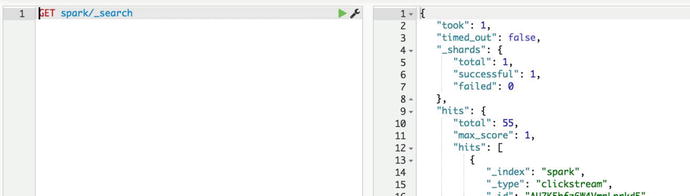
Figure 5-3. Clickstream events in the spark index
As you can see, I’m using Elasticsearch search API to fetch data from the spark index; as a result, I’m getting 55 clickstream events from the index.
Implementing a Spark Data Processing
That may look weird to end with part, but I prefer that the streaming to pipe be ready to work before diving on the core usage of Spark, the data processing.
We will now add a little bit more processing logic to our previous Spark code and introduce a new object: the PageStatistic object. This object will hold all the statistics that we want to have around user behavior on our website. We’ll limit the example to a basic one; in the next chapter, we’ll will go deeper.
The processing part will be then be divided into the following parts:
- creation on a simple PageStatistic object that holds the statistics
- computation of statistic
- indexation part
Let’s first begin with the PageStatistic object, which so far will only hold the count of GET and POST request, as shown in Listing 5-24.
Then we’ll use a special from Spark scala library call countByValue to compute the number of GET and POST in the batch of logs we receive from Kafka as seen in Listing 5-25.
In this code, we simply take each received event and apply the countByValue function on it. Then we create a map with a default value of 0, which we iterate on to pull out PageStatistic objects.
Finally, we index the data in Elasticsearch using the spark index and create a new type of document, the stats, as seen in Listing 5-26.
If we check in Elasticsearch using Listing 5-27:
We get:
{
   "took": 1,
   "timed_out": false,
   "_shards": {
      "total": 1,
      "successful": 1,
      "failed": 0
   },
   "hits": {
      "total": 1,
      "max_score": 1,
      "hits": [
         {
            "_index": "spark",
            "_type": "stats",
            "_id": "AU7ReZIVvtspbVGliqwM",
            "_score": 1,
            "_source": {
               "getRequest": 34,
               "postRequest": 12
            }
         }
      ]
   }
}
We can see that our document holds the two computed fields of the PageStatistic object. But this level of trivial computation is something that Elasticsearch can easily do; we’ll see how in the next section. Remember that we’ll try to emphasize this Spark processing pipeline in the following chapter, to show the full power of this stack.
Data Analytics with Elasticsearch
Introduction to the aggregation framework
Elasticsearch comes with a powerful set of API that let the users get the best of their data. The aggregation framework groups and enables real-time analytics queries on small to large set of data.
What we have done with Spark in terms of simple analytics can be done as well in Elasticsearch using the aggregation framework at scale. This framework is devided into two types of aggregations:
- Bucket aggregation that aims to group a set of document based on key common to documents and criterion. Document that meets the condition falls in the bucket.
- Metric aggregation that aims to calculate metrics such as average, maximum, minimum, or even date histograms, over a set of documents.
Indeed, the power of aggregation resides on the fact that they can be nested
Bucket Aggregation
Bucket aggregation is used to create groups of documents. As opposed to metric aggregation, this can be nested so that you can get real-time multilevel aggregation. Whereas in Spark creating the PageStatistic structure needed a bunch of coding and logic that would differ from a developer to the other, which could affect the performance of the processing dramatically, in Elasticsearch there is less work to reach the same target.
The bucketing aggregation is really easy to implement. Let’s take an example of verb distribution; if we want to group document per verb, all we have to do is follow the code shown in Listing 5-28.
Which then returns the code shown in Listing 5-29.
As you can see, I’m running the aggregation in couple of milliseconds, so near real time (11 ms) and getting the distribution of get and post HTTP verbs. But what if we want to get an equivalent result that we had in Spark, a time-based distribution of HTTP verbs? Let’s use the date histogram aggregation and have a nested term aggregation into it, as shown in Listing 5-30.
The date histogram aggregation is indeed really easy to use; it specifies:
- The field holding the timestamp that the histogram will use
- The interval for bucketing. Here I’ve used minute because I’m indexing more than 1 million documents on the laptop while I’m writing this book. This obviously takes time so I’m sure to have document distributed over minutes. I could have used day, month, or year, or specified a date expression 2h for “every 2 hours”.
You see the nested term aggregation in my query; let’s just switch the interval to 20m for getting a more condensed result, shown in Listing 5-31.
As you can see, we get two buckets of 20 minutes data and the nested distribution of HTTP verbs. This kind of aggregation is ideal when you want to draw them as timelines or bar charts that render the data over time with a fine control of the period of time you want to analyze the data.
Let’s now see what happen if we use a metric aggregation.
Metric Aggregation
Metric aggregations are the last level of set of aggregation and are use to compute metrics over set of documents. Some of the computations are considered as single value metric aggregation because they basically compute a specific operation across document such as average, min, max or sum, some are multi-value aggregation because they give more than one statistic metrics for a specific field across documents such as the stats aggregation.
As an example of multivalue aggregation metric, let’s make a stats aggregation on the bytes field to get more visibility on the throughput of our website page, with Listing 5-32.
The stats aggregation only takes a numeric field as input—here, bytes—and returns Listing 5-33.
The results give the computation of differents metrics for the bytes field:
- The count represents the number of documents the query has been on, here more than 2.5 million
- The min & max are respectively the minimum and maximum of bytes
- The avg is the average bytes value for all documents
- The sum is the sum of all bytes field across documents
This is how you can with a small query extract statistic from your document, but let’s try to go further and combine our bucket and metric aggregation. What we will try to do is to add another level of aggregation and check what is the throughput on each of HTTP verb type, shown in Listing 5-34.
We will get the bytes statistics for each HTTP verb every 20 minutes, as shown in Listing 5-35.
The point here is not to redo what Spark does, for this type of operation Elasticsearch is handier; the goal is to use those features to leverage what Spark can do.
Visualize Data in Kibana
As an example of a resulting report, we will create a Kibana 4 dashboard that shows how Elasticsearch aggregation API is used.
The Kibana UI is accessible on your local installation via the following URL:
http://localhost:5601
In Kibana discovery tab, we can see that we are receving data, as shown in Figure 5-4.
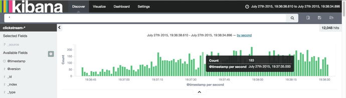
Figure 5-4. Discovering clickstream data
Let’s try to make a bar chart visualization that shows the distribution of HTTP response code over time. This can lead to anomaly detection such as intrusion attempt on our website and so on.
The visualization tab lets you create by configuration this kind of charts, as shown in Figure 5-5.
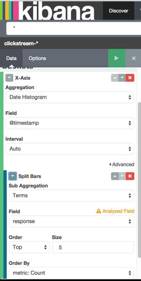
Figure 5-5. Creating aggregation in Kibana
What we expect is for Kibana to draw a report that shows the number of 200, 404, and so on over time, as shown in Figure 5-6.
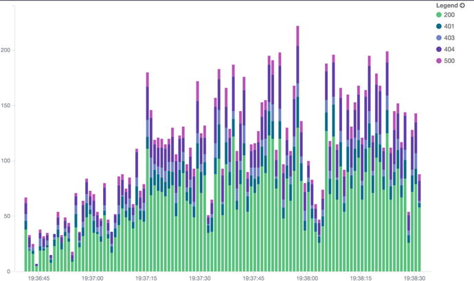
Figure 5-6. HTTP response code over time
Visualizing our data brings us to another dimension and easily shows the power of the aggregation framework. Kibana doesn’t compute anything on its side; it just renders the data that are returned from Elasticsearch. Listing 5-36 shows what Kibana is asking under the hood.
Kibana is relying on Elasticsearch scaling ability and those kinds of visualizations can be done on small to very large sets of data. In the end, what you want to get is a complete view of your data, such as the Kibana dashboard shown in Figure 5-7.
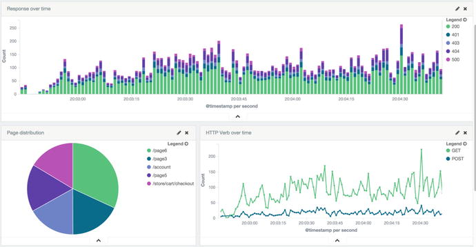
Figure 5-7. Kibana dashboard
Summary
In the next chapter, we’ll add more complexity to our processing and bring more prediction to it. In addition, we’ll continue to illustrate the results of processing with Kibana dashboard.