12
Evaluating, Recommending, and Presenting Your Solutions
We started our journey with the basics of data engineering and learned various ways to solve data ingestion and data publishing problems. We learned about various architectural patterns, as well as the governance and security of the solution. In the preceding chapter, we discussed how we can achieve performance engineering and how to create a performance benchmark for our solution.
By now, we have acquired multiple skills to architect efficient, scalable, and optimized data engineering solutions. However, as discussed in the Responsibilities and challenges of a Java data architect section of Chapter 1, Basics of Modern Data Architecture, a data architect has multiple roles to play. In an executive role, the data architect becomes the bridge between business and technology who can communicate ideas effectively and easily with the respective stakeholders. An architect’s job is not only to create the solution but also to present and sell their idea to executives and leadership (both functional and technical). In this chapter, we will focus on how to recommend and present a solution.
In this chapter, we will start our discussion by talking about infrastructure and human resource estimation. As data architects, we need to recommend solutions. To do that, we will discuss how we can create a decision matrix to evaluate our solution and compare different alternatives. Then, we will learn about using decision charts effectively to choose an optimal architectural alternative. Finally, we’ll learn about a few basic tips and tricks to present the solution effectively.
In this chapter, we’re going to cover the following main topics:
- Creating cost and resource estimations
- Creating an architectural decision matrix
- Data-driven architectural decisions to mitigate risk
- Presenting the solution and recommendations
Creating cost and resource estimations
In this section, we will discuss various considerations, methods, and techniques that we apply to create estimations. We will briefly discuss both infrastructure estimations as well as human resource estimations. Infrastructure estimations are closely related to capacity planning. So, we will start our discussion with capacity planning.
Storage and compute capacity planning
To create an infrastructure estimate, you have to find out the data storage needs (RAM, hard disks, volumes, and so on) and the compute needs (the number of CPUs/vCPUs and cores it should have). This process of figuring out the storage and compute needs is called capacity planning. We will start by learning about the factors that need to be considered while conducting capacity planning.
Factors that need to be considered while conducting capacity planning
The following are the various factors that should be taken into consideration while creating a capacity plan:
- Input data rate: Based on the type of application, data rates need to be factored in. For example, for a real-time or near-real-time application, the peak data rate should be considered while planning for the storage and compute capacity. For batch-based applications, either the median data rate or the average data rate should be considered. If the batch job runs daily, it is advisable to use median data rates for capacity planning. Median data rates are preferred over average data rates because median data rates are based on the densest distribution of data rates. So, it denotes the middle point of the most frequently recorded data rate. Hence, the median value is never affected by any outlier. On the other hand, the average data rate finds the average of all the data rates over time, including a few exceptional high or low data rates.
- Data replication and RAID configurations: Replication ensures high availability and data locality. Since it replicates the data to multiple nodes, systems, or partitions, we must consider the replication factor as well while planning for storage capacity. For example, if 5 GB of data is stored with a replication factor of 3, this means it stores two replicas in different systems, along with the original message. So, the total storage requirement to store 5 GB of data is 15 GB. The replication factor is often mistaken for RAID. While the replication factor ensures high availability using data locality, RAID ensures data safety at the physical storage level by ensuring redundancy at the storage array layer. For mission-critical use cases, it is advisable to take both replication and RAID into consideration while planning for storage capacity.
- Data retention: Another important factor is data retention. Data retention is the time for which data needs to be retained in storage before it’s purged. This plays an important role as it determines how much storage is needed for accumulation purposes. One of the other things that comes into play in the cloud is the need for archival. Does data need to be archived? If that’s true, when should it be archived?
Initially, data may be frequently accessed. Then, it can be infrequently accessed, and the company may want to store the data in an archival zone for long-term audit and reporting requirements. Such a scenario can be handled in the cloud by using specific strategies to save money. For example, we can use S3 intelligent tiering, which sends the data automatically from the S3 standard access to S3 infrequent access layers to the S3 Glacier layers based on the access frequency. This reduces Operating Expenses (OpEx) costs as you can make a lot of savings as you move your data from the standard access layer to Glacier.
- Type of data platform: It also matters whether you are running your application on-premises or in the public cloud. Capacity planning should consider the maximum required capacity while planning for on-premise deployment. But if you are planning for the cloud, it is advisable to go with a median capacity requirement and configure auto-scaling for peak loads. Since the cloud gives you the option of instant scaling as well as paying for only what you use, it makes sense to spin up the resources required to process the usual data volumes.
- Data growth: Another thing you must consider is the growth rate of data. Based on various factors, growth rates may vary. It is important to factor in the growth rate since data engineering pipelines are usually long-term investments.
- Parallel executions in shared mode: One of the other factors that we must take into account is shared resources and their effect on concurrent executions. For example, it helps us to correctly estimate the resource requirement of a big data cluster if we know that 10 jobs with an average approximate load of 100 GB may run simultaneously on the cluster. Similarly, to estimate the resource requirements of a Kubernetes cluster, we should be aware of the maximum number of pods that will be running simultaneously. This will help determine the size and number of physical machines and VMs you want to spawn.
With that, we have learned about the various factors that need to be considered while doing storage and compute capacity planning. In the next section, we will look through a few examples of how these factors help in capacity planning.
Applying these considerations to calculate the capacity
In this section, we will discuss a few examples where the aforementioned factors are used judiciously to calculate capacity. The following are a few use cases:
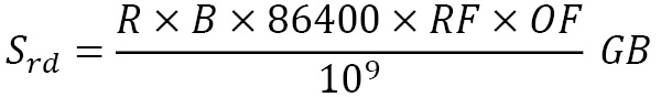
- Example 1: Consider that we need to create a capacity plan for a big data cluster in an on-premise data center. Here, the input data rate is R records per second and each record is B bytes. The storage requirement for a day (
 ) can be calculated by multiplying R by B and multiplying the result by 86,400 seconds. However, this calculation doesn’t include the replication or RAID factors. We must multiply the replication factor (here, RF) by it, as well as the overload factor (here, OF), due to RAID configurations (the overload factor for RAID 0 is 1, RAID 5 is 1.5, and RAID 10 is 2). Hence, the formula to calculate the storage requirements for a day is as follows:
But the actual capacity requirement may be more than this. If there is a requirement to retain data for 7 days, we will get the total required storage by multiplying 7 by  . Now, let’s see how the growth factor can affect capacity planning. Based on the technology stack, volume of data and data access, and read pattern and frequency, we can set the total memory and compute. Let’s say that the calculated storage capacity is
 ![]() , memory is
, memory is ![]() , compute is
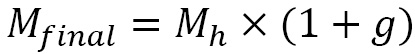
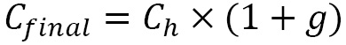
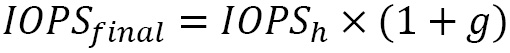
, compute is ![]() , and Input/Output Operations per Second (IOPS) is
, and Input/Output Operations per Second (IOPS) is  . Also, let’s say that the growth rate is g per year. So, the final resource requirement for the next year would be as follows:
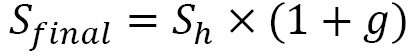
In this example, we saw how our factors help size a Hadoop big data cluster. Hardware Capital Expenditure (CapEx) represents a significant investment upfront and requires recurring OpEx, hence a balance between the two needs to be attained for better TOC.. In the next example, we’ll explore how to size a Kafka cluster for real-time loads.
- Example 2: In this example, we are trying to predict the capacity of a Kafka cluster that receives 100 messages per second, where the retention period is 1 week and the average message size is 10 KB. Also, all topics have a replication factor of 3. Here, a Kafka cluster contains two primary clusters – a Kafka cluster and a zookeeper cluster. For a zookeeper cluster in production, a dual-core or higher CPU should be used, along with a memory of 16 to 24 GB. 500 GB to 1 TB disk space should be fine for zookeeper nodes. For the Kafka broker nodes, we should run multi-core servers with 12 nodes and higher. It should also support hyperthreading. The usual normal memory requirement for a Kafka broker is between 24 to 32 GB. Now, let’s calculate the storage needs for the broker. The following formula helps calculate the storage needs for each node:
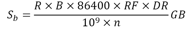


By applying this formula to our example, we get the storage needs of each broker as 604 GB.
With these examples, we’ve seen how we can apply various factors to predict the capacity requirement of a solution. This helps create detailed CapEx and OpEx estimations for the business.
Now that we have learned how infrastructure estimations are calculated, we will discuss how to estimate the human resource-related costs and time for executing a project.
Effort and timeline estimation
Apart from the various responsibilities that an architect has to handle, effort and time estimation is an important responsibility for a data architect. Usually, the architect is responsible for creating a high-level estimate at the start of the project’s implementation. Considering most teams follow the agile methodology of software development, detailed effort estimation is done by the agile team during the implementation phase. The following activities need to be done to create a good estimate:
- Create tasks and dependency charts: First, to create an estimate, we must analyze the solution and divide it into high-level development and quality assurance tasks. We should also factor in all performance engineering tasks while creating the high-level task list. Then, we must create a dependency task list, which will specify whether a particular task is dependent on another task(s) or not. The following table shows one of the formats for creating a task and dependency list:
|
Task no. |
Task name |
Dependency |
|
1 |
Creating Git user registration and a master repository | |
|
2 |
Creating local repositories on a PC |
Task 1 |
|
3 |
Creating a simple Hello World whose output will be shown in Hindi in Java | |
|
4 |
Creating R2 | |
|
5 |
Reviewing the code of R2 |
Task 4 |
|
6 |
Pushing the code of R2 |
Task 2 and Task 5 |
|
7 |
Creating a data model of R2 | |
|
8 |
Creating a data model of R3-b | |
|
9 |
Reviewing the data model of R3-b |
Task 8 |
|
10 |
Pushing the data model of R3-b |
Task 1 and Task 8 |
Figure 12.1 – Sample task and dependency list
In the preceding table, note that task 2 is dependent on task 1 and, similarly, task 6 is dependent on tasks 2 and 5. Note how we can denote such dependencies by adding a dependency column. This dependency matrix helps us understand the risks and dependencies. It also helps us understand how various tasks can run in parallel. This helps create a roadmap for various feature releases.
- Classify the tasks based on their complexity: One of the things that an architect must do is classify the tasks into one of three categories: high complexity, medium complexity, and low complexity. However, for some exceptional use cases, more granular complexity levels can be defined.
- Classify based on technology: Another classification that helps with estimation is technology. This is because a complex task for a Spark-based job can be different than a complex task for a DataStage-based job. So, the average effort that needs to be spent not only depends on the complexity but also on the technology.
- Create the estimated time taken for a task: To create a time estimate, first, we must create a map consisting of the time taken for a specific combination of technology and complexity if it is a technical task. If it is an analytical task, we must create a mapping for the time taken by a task versus its complexity. For example, a complex task for a Spark job may take 8 man-days to finish, while a complex task for an Informatica job may take 5 man-days to finish. Based on such a mapping, we can estimate the total time taken to finish the project in man-days or man-hours. For some agile projects, this effort can be estimated using a point system. For example, a complex analysis task may take 5 points of effort.
- Create total effort estimates: Based on the estimation done in the previous steps, we can calculate the total effort by summing up all individual task efforts required to deliver the solution.
- Add a buffer to estimates: As mentioned in the book The Pragmatic Programmer (Hunt et al., 1999), we should remember that Rather than construction, software is more like gardening – it is more organic than concrete. You constantly monitor the health of the garden and make adjustments (to the soil, the plants, the layout) as needed. Since developing any application or data pipeline is organic, we must add a buffer to our estimates so that any organic changes may be accommodated in the project schedule.
- Create a product roadmap and timeline for releases: Based on the total estimate, dependency, risks, and expected delivery range, we can create a roadmap and timeline. It is important to understand the expected delivery timelines to ensure we can do proper resource loading and deliver the project in the time range that the business is looking for. Having said that, a lot of times, the business has unrealistic expectations of delivery timelines. It is the job of an architect (with the help of the project manager and product owner) to communicate and justify the estimates to the business so that both the technical and business teams can come to a common ground in terms of the delivery timeline.
- List all risks and dependencies alongside the estimate: While creating an estimate, it is important to list all the risks, dependencies, and assumptions so that all stakeholders are aware of what is being delivered and the risks involved in delivering the solution.
Now that we have learned how to create and document a well-thought effort estimate, we have to figure out the total delivery or development cost of a solution. To do that, we must perform human resource loading. Human resource loading is a process by which we identify how many developers, testers, and analysts with specific skill sets are required to deliver the project in the agreed-upon time. Finding the right mix of people with specific roles is the key to delivering the solution. Then, we assign a specific per-hour cost based on the role, demographics, and technology.
After that, we factor in the number of hours required by a role or resource and multiply it by the assigned rate to reach the total cost of a human resource for the project. By summing up the total cost of each resource, we can find the total development cost (or the labor cost; any infra or license costs are not included).
With that, we have learned how to create cost and resource estimates to implement a solution. Earlier in this book, we learned how to develop different architectures for various kinds of data engineering problems. We also learned how to run performance tests and benchmarks.
In this section, we learned how to create cost and resource estimates to implement a solution. Is there a way to stitch all this information together to recommend the best-suited solution? In real-world scenarios, each data engineering problem can be solved by multiple architectural solutions. How do we know which is the most suitable solution? Is there a logical way to determine the best-suited solution? Let’s find out.
Creating an architectural decision matrix
Concerning data engineering, an architectural decision matrix is a tool that helps architects evaluate the different architectural approaches with clarity and objectivity. A decision matrix is a grid that outlines the various desirable criteria for making architectural decisions. This tool helps rank different architectural alternatives, based on the score for each criterion. Decision matrices are used by other decision-making processes. For example, decision matrices are used by business analysts to analyze and evaluate their options.
The decision matrix, also known as the Pugh matrix, decision grid, or grid analysis, can be used for many types of decision-making processes. However, it is best suited for scenarios where we have to choose one option among a group of alternatives. Since we must choose one architecture for the recommendation, it makes sense to use a decision matrix to arrive at a conclusion. Now, let’s discuss a step-by-step guide to creating a decision matrix for architectural decision-making. The steps to create a decision matrix are as follows:
- Brainstorm and finalize the various criteria: To create a decision matrix that can be used for architectural evaluation, it is important to brainstorm and finalize the various criteria that the decision depends on. It is important to involve leadership and business executives as stakeholders in this brainstorming session. If you are an architect from a services firm who is developing a solution for the client, it is important to involve an architect from the client side as well. This step is very important as various criteria and their priorities help narrow down our final recommendation among a set of architectural alternatives.
- Create the matrix table: Next, we should create the decision matrix table, where each row denotes a specific criterion, while each column denotes a specific architectural alternative. These are selected sets of criteria that help us determine the appropriateness of the architecture for the current use case. The following diagram shows what the table will look like:
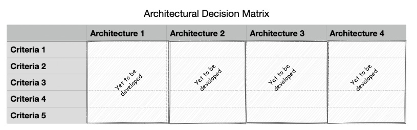
Figure 12.2 – Creating the decision matrix table
- Assign rank or scale: Now, we must assign rank or scale to each of the criteria of the architecture. Rank or scale is a relative measure where the higher the scale, the better it fits the criteria. The following diagram shows how scale is assigned to different architectures based on various criteria:
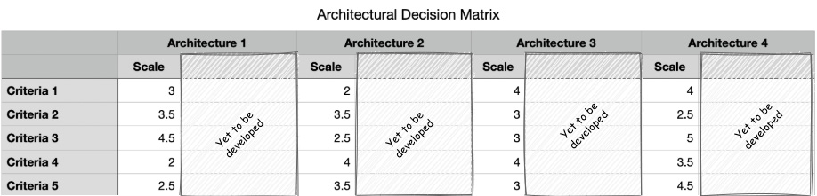
Figure 12.3 – Assigning scale values for each architecture against each criterion
As we can see, different scales are assigned to each architecture against each criterion on a relative scale of 1 to 5. Here, 5 is the highest match possible for the given criterion, while 1 is the lowest match possible for the given criterion. In this example, Architecture 1 gets a score of 3 in terms of Scale. Architecture 2 gets a score of 2, while Architecture 3 and Architecture 4 get a score of 4 for Criteria 1. Hence, Architecture 3 and Architecture 4 are the most suitable as far as Criteria 1 is concerned.
- Assign weights: Next, we must assign weights to each criterion. This will help set the priority for various criteria. The following diagram shows how weights are assigned to each architecture against each criterion:
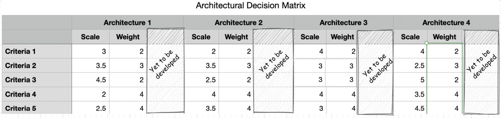
Figure 12.4 – Assigning weights to each criterion
As we can see, the weight that’s assigned to each criterion is independent of the architecture. This attaches a priority to each of the criteria. So, the most desirable criteria get the highest preference. The higher the weight, the higher the priority. In this example, Criteria 1 and Criteria 2 get the least priority with a priority score of 2, while Criteria 4 and Criteria 5 get the highest priority with a priority score of 4.
- Calculate the score: The individual scores for each architecture against a criterion are calculated by multiplying scale values by the weight of the criteria. The total desirability score of the architecture is calculated by summing up all the scores of each criterion. The following diagram shows what such a decision matrix looks like:
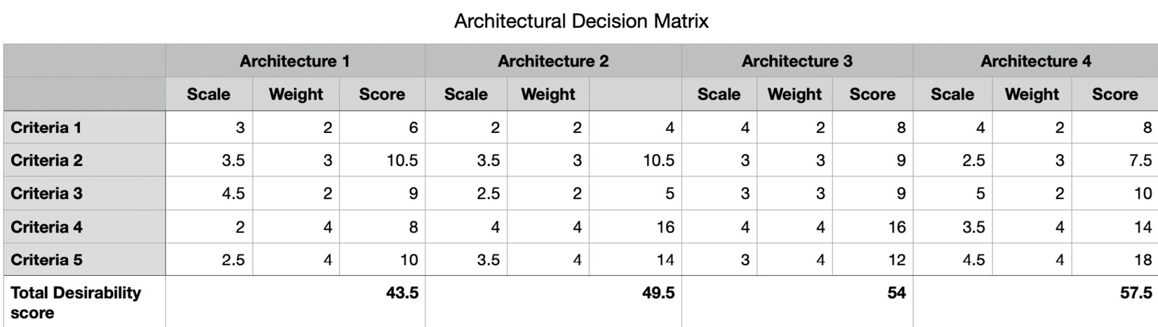
Figure 12.5 – Example of a completed decision matrix for architectural decisions
As we can see, Architecture 4 looks like the most desirable solution as it has the highest total desirability score of 57.5, while Architecture 1 is the least desirable with a score of 43.5.
In this section, we learned about how to create a decision matrix. Now, the question is, is the total desirability score always enough to recommend an architecture? In the next section, we’ll learn how to further evaluate an architecture by using the techniques we learned earlier.
Data-driven architectural decisions to mitigate risk
A decision matrix helps us evaluate the desirability of an architecture. However, it is not always necessary to opt for the architectural option that has the highest desirability score. Sometimes, each criterion needs to have a minimum threshold score for an architecture to be selected. Such scenarios can be handled by a spider chart.
A spider chart, also known as a radar chart, is often used to display data across multiple dimensions. Each dimension is represented by an axis. Usually, the dimensions are quantitative and normalized to match a particular range. Then, each option is plotted against all the dimensions to create a closed polygon structure, as shown in the following diagram:
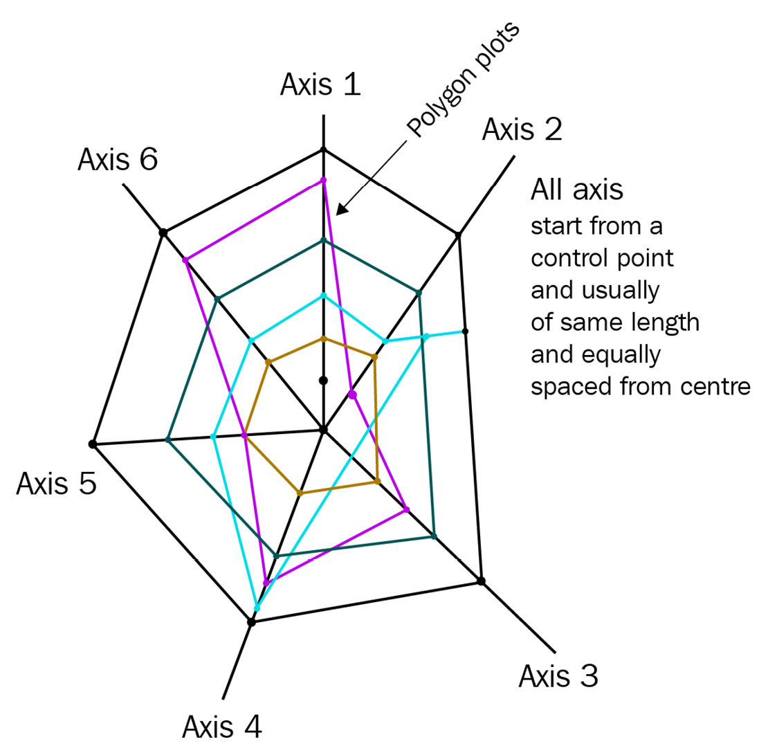
Figure 12.6 – Spider or radar chart
In our case, each criterion for making an architectural decision can be considered a dimension. Also, each architectural alternative is plotted as a graph on the radar chart. Let’s look at the use case for the decision matrix shown in Figure 12.5. The following diagram shows the radar chart for the same use case:
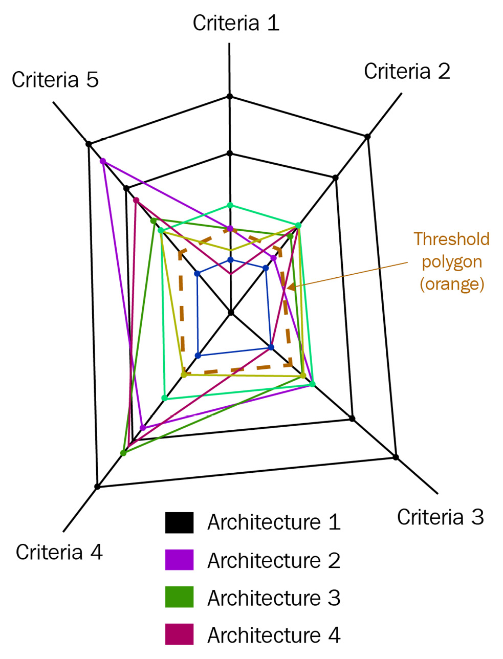
Figure 12.7 – Radar chart for the example scenario discussed earlier
As we can see, each axis denotes a criterion such as Criteria 1, Criteria 2, and so on. Each criterion has a total score of 25 points, divided into five equal parts along its axis. The division markers for each criterion are connected to the division marker of the adjacent criteria, creating a spider web of symmetrical pentagons. The maximum score of each criterion is 25 because it is the product of the maximum scale value (5) and the maximum weightage (5). We also create a threshold polygon, as denoted by the dotted lines in the preceding diagram. This is created by joining the threshold marker (in this case, a score of 8 points) for every criterion. An optimal solution is one whose polygon is either bigger or equal to the threshold polygon. All the criteria of an optimal solution should score more points than the threshold score of each criterion.
As shown in the preceding diagram, our threshold score for each criterion is 8. Based on the score of each criterion for the architecture, we draw the polygon plot. Here, the plot of Architecture 1 is blue, Architecture 2 is pink, Architecture 3 is green, and Architecture 4 is violet. Based on the plots, we can see that only Architecture 3 is optimal in this use case. Although the total desirability score of Architecture 4 is greater than that of Architecture 3, it doesn’t fulfill the condition of having the minimum threshold score of 8 for each criterion as it only scores 7.5 in Criteria 2. Also, if the individual score of each criterion for Architecture 3 is more than or equal to the threshold score. Hence, Architecture 3 is the best-suited option for this use case.
An alternative way to evaluate a decision matrix to find the most optimized solution is using a decision tree. Decision trees are decision support tools that use tree-like models for questions and categorize or prune the results based on the answer to those questions. Usually, the leaf nodes denote the category or the decision. The following diagram shows an example of a decision tree for evaluating the scenario that we just discussed using a spider/radar chart:
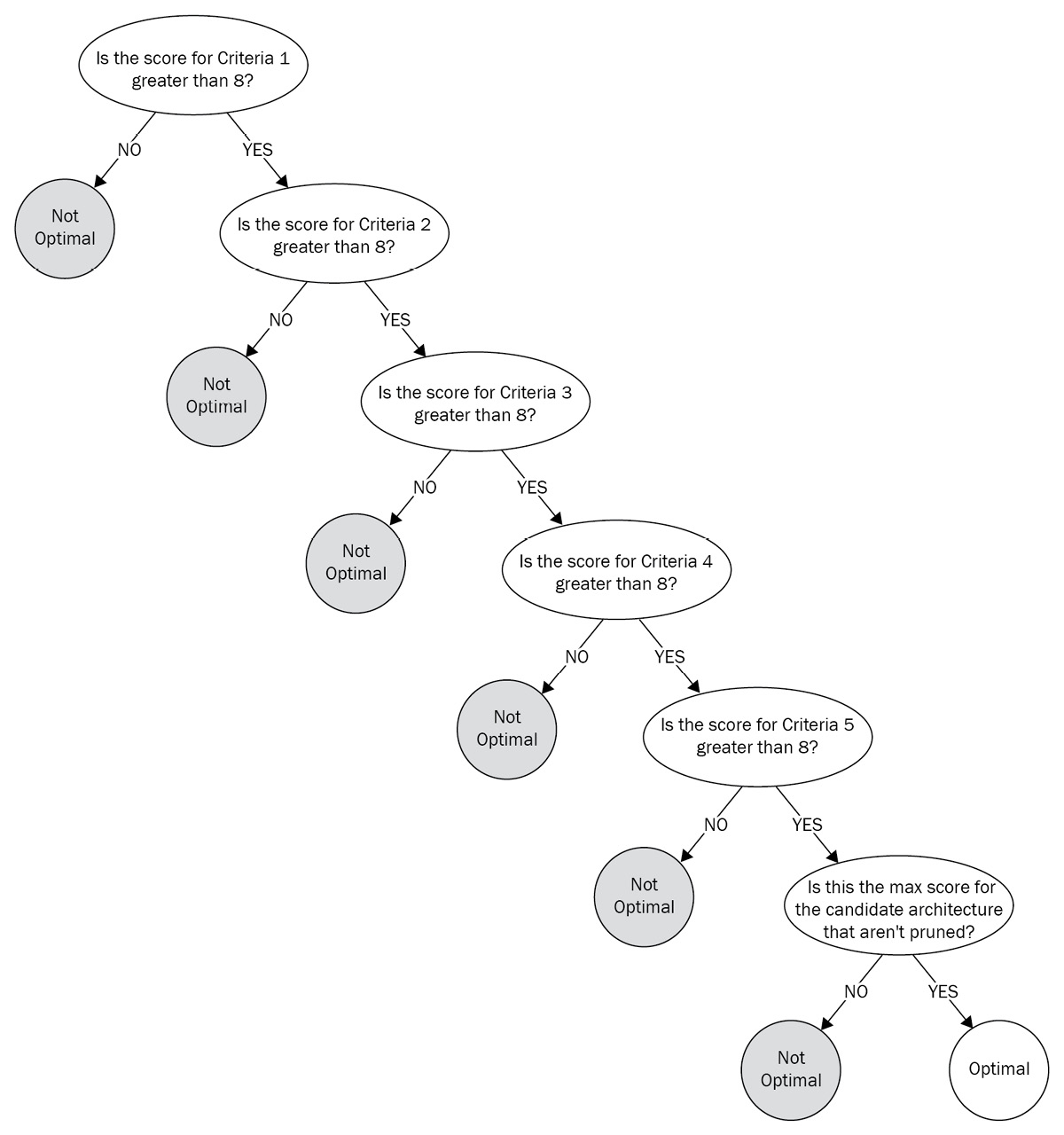
Figure 12.8 – Decision tree to evaluate architectural alternatives
As we can see, we can create a decision tree based on the scores recorded earlier in the decision matrix to find the most optimal solution. Here, we are asking questions such as Is the score for Criteria 1 greater than 8?, Is the score for Criteria 2 greater than 8?, and so on. Based on the answer, we are pruning out the non-optimal solutions at that level. Finally, we ask, Is this the max score for the candidate architecture and it can’t be pruned? The answer to this question helps us figure out the most optimal solution.
In this section, we learned how to use a data-driven methodical approach to find and evaluate the most optimal solution for the problem. Now, it is the job of the architect to present the solution as a recommendation. In the next section, we will discuss the guidelines for how to present your solution effectively.
Presenting the solution and recommendations
As an architect, your job doesn’t end when you create and evaluate the most optimal architectural alternative based on the problem, platform, criteria, and priorities. As a Janus between business and technology, the architect is also responsible for effectively communicating the solution and recommending the most optimal alternative. Based on the kind of project and the type of business you are in, you may be required to convince stakeholders to invest in the solution. The following are a few guidelines that will help you present your solution and convince your stakeholders more effectively:
- Present the presentation before the presentation: If possible, engage the customer or end client early and give them a glimpse of what possible solutions you are thinking of. Also, tell them how much time will it take for you to evaluate each of the solutions. Keep them engaged and in the loop while developing the architecture. It is always helpful if stakeholders are involved in the process and kept in the loop. It’s a win-win situation for both the stakeholders and the architect. Stakeholders feel that they are part of the solution, and they get enough time to understand or anticipate any impact of implementing the solution. On the other hand, the architect gets constant feedback about the priorities and criteria, which helps them come up with a very well-researched decision matrix. A more accurate decision matrix eventually helps architects make the most desired recommendation.
- Know your audience and ensure they are present: Although this is true for any presentation, it is important to understand the audience before presenting the solution. It is important to understand whether they are from business, executive leadership, or the technical side. It is also important to consider if any external teams or vendors are involved. Understanding the demographics of your audience will help you customize your presentation so that it is relatable to their work. If it is a mixed audience, make sure that you have something relatable for all the different audience groups. It is also important that you invite all the important stakeholders so that your solution reaches every intended audience.
- Present the Return on Investment (ROI) for the solution: Usually, there are top-level leaders, executives, and business heads present in a solution presentation. For them, it is important to understand how the solution can either generate or save dollars. It could be that the solution will create additional revenue generation sources, or it could be as trivial as a lesser total cost of ownership or a lesser cost of development. To showcase the ROI for the solution, you can include if the solution adds any value to the customer experience or acceptance of the product. A good data architect should carefully brainstorm and figure out how the solution can add value to the business.
- Recommend by comparing alternatives: Although we, as architects, usually recommend one architecture, it is a good practice to present all the alternative architectures and their pros and cons. Then, we must establish the most suitable architecture. It is also a good idea to present why we chose that architecture.
- Make the presentation better by using their language: Each company and business has its own language. Since a lot of stakeholders are from the business side of things, it is better to adapt to the common language that’s popular in the organization when presenting. This ensures that the audience is easily getting what we are presenting and can connect the dots.
- Mind the context: It is also important for the presentation to be contextual. Based on the audience, your presentation should be customized so that it has the correct balance between technical versus business content.
- Ensure your presentation is visually appealing and relatable: Diagrams speak more than words. Presentations must have clear diagrams that are relatable and self-explanatory. Avoid too much text in a presentation. A visually appealing presentation is easier to explain and keeps the various stakeholders interested in the presentation.
In this section, we discussed a few tips and tricks for presenting a solution to stakeholders in a concise, effective, and impactful way. Apart from developing and architecting a solution, we are aware of how to evaluate, recommend, and present a solution effectively. Now, let’s summarize what we learned in this chapter.
Summary
We started this chapter by learning how to plan and estimate infrastructure resources. Then, we discussed how to do an effort estimation, how to load human resources, and how to calculate the total development cost. By doing so, we learned how to create an architectural decision matrix and how to perform data-driven comparisons between different architectures. Then, we delved into the different ways we can use the decision matrix to evaluate the most optimal solution by using spider/radar charts or decision trees. Finally, we discussed some guidelines and tips for presenting the optimized solution in a more effective and impactful way to various business stakeholders.
Congratulations – you have completed all 12 chapters of this book, where you learned all about a Java data architect’s role, the basics of data engineering, how to build solutions for various kinds of data engineering problems, various architectural patterns, data governance and security, and performance engineering and optimization. In this final chapter, you learned how to use data-driven techniques to choose the best-suited architecture and how to present it to the executive leadership. I hope you have learned a lot, and that it will help you develop your career as a successful data architect and help you grow in your current role.