
Static web serving doesn’t seem so difficult at first. And, in truth, it isn’t. However, as sites evolve and grow, they must scale, and the stresses of serving traffic in development and staging are different from those placed on an architecture by millions of visitors.
Let’s walk through a typical approach to serving a website and then investigate that approach for inefficiencies. First, how much of the traffic is static? The answer to this is the basis for numerous timing, throughput, and other scalability calculations. Table 6.1 shows four sites: three real sites (one very small site and two that are huge) and a fourth site that is an example large site for discussion purposes whose page composition metrics are legitimized by the real data.
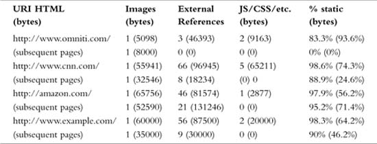
As can be seen in Table 6.1, the number of requests for static content far outweighs the number of requests for possibly dynamic HTML pages. Additionally, the volume of static content served constitutes more than 50% of the total volume served.
Although browser cache reduces the number of queries for these static objects (particularly images) as can be seen in the “subsequent pages” rows, it does not eliminate them entirely. Sites that rarely change will benefit tremendously from browser-side caching, whereas other more dynamic sites will not. If you look at a popular online news source (such as CNN or BBC), you will notice that almost every news story that is added contains several new external objects whether an image, movie, or audio stream. As visitors come, they are unlikely to reread the same article, and thus unlikely to capitalize on the existence of the corresponding images in their browser’s cache. While surfing on the CNN site, I calculated about an 88% cache hit rate for static objects within a page.
Additionally, ISPs, corporations, and even small companies employ transparent and nontransparent caching web proxies to help reduce network usage and improve user experience. This means that when Bob loads a page and all its images, Bob’s ISP may cache those images on its network so that when another user from that ISP requests the page and attempts to fetch the embedded images, he will wind up pulling them (more quickly) from the ISP’s local cache.
Where does this leave us? When a user first visits www.example.com, what happens on the network level? When I point my browser at www.example.com, it attempts to open seven TCP/IP connections to download the HTML base page and all the subsequent stylesheets, JavaScript includes, and images. Additionally, these seven connections are open for an average of 4 seconds.
Now, it should be obvious that only one of those TCP/IP connections was used to fetch the base document as it was fetched first and only once, and that the connection was reused to fetch some of the static objects. That leaves six induced connections due to page dependencies. Although subsequent page loads weren’t so dramatic, the initial page loads alone provide enough evidence to paint a dismal picture.
Let’s take the most popular web server on the Internet as the basis for our discussion. According to NetCraft web survey, Apache is the web server technology behind approximately 67% of all Internet sites with a footprint of approximately 33 million websites. It is considered by many industry experts to be an excellent tool for enterprise and carrier-class deployments, and it has my vote of confidence as well. For a variety of reasons, Apache 1.3 remains far more popular than Apache 2.0, so we will assume Apache 1.3.x to be core technology for our web installation at www.example.com.
Apache 1.3 uses a process model to handle requests and serve traffic. This means that when a TCP/IP connection is made, a process is dedicated to fielding all the requests that arrive on that connection—and yes, the process remains dedicated during all the lag time, pauses, and slow content delivery due to slow client connection speed.
How many processes can your system run? Most Unix-like machines ship with a maximum process limit between 512 and 20,000. That is a big range, but we can narrow it down if we consider the speed of a context switch. Context switching on most modern Unix-like systems is fast and completely unnoticeable on a workstation when 100 processes are running. However, this is because 100 processes aren’t running; only a handful is actually running at any given time. In stark comparison, on a heavily trafficked web server, all the processes are on the CPU or are waiting for some “in-demand” resource such as the CPU or disk.
Due to the nature of web requests (being quick and short), you have processes accomplishing relatively small units of work at any given time. This leads to processes bouncing into and out of the run queue at a rapid rate. When one process is taken off the CPU and another process (from the run queue) is placed on the CPU to execute it, it is called a context switch. We won’t get into the details, but the important thing to remember is that nothing in computing is free.
There is a common misconception that serving a web request requires the process to be switched onto the processor, where it does its job, and then gets switched off again, requiring a total of two context switches. This is not true. Any time a task must communicate over the network (to a client or to a database), or read from or write to disk, it has nothing to do while those interactions are being completed. At the bare minimum, a web server process must
Each of these actions requires the process to be context switched in and then out, totaling 10 context switches. If multiple requests are serviced over the life of a single connection, the first and last events in the preceding list are amortized over the life of the connection, dropping the total to slightly more than six. However, the preceding events are the bare minimum. Typically, websites do something when they service requests, which places one or more events (such as file I/O or database operations) between reading the request and writing the response. In the end, 10 context switches is a hopeful lower bound that most web environments never achieve.
Assume that a context takes an average of 10μ (microseconds) to complete. That means that the server can perform 100,000 context switches per second, and at 10 per web request that comes out to 10,000 web requests per second, right? No.
The system could perform the context switches necessary to service 10,000 requests per second, but then it would not have resources remaining to do anything. In other words, it would be spending 100% of its time switching between processes and never actually running them.
Well, that’s okay. The goal isn’t to serve 10,000 requests per second. Instead, we have a modest goal of serving 1,000 requests per second. At that rate, we spend 10% of all time on the system switching between tasks. Although 10% isn’t an enormous amount, an architect should always consider this when the CPU is being used for other important tasks such as generating dynamic content.
Many web server platforms in use have different design architectures than Apache 1.3.x. Some are based on a thread per request, some are event driven, and others take the extreme approach of servicing a portion of the requests from within the kernel of the operating system, and by doing so, help alleviate the particular nuisance of context switching costs.
As so many existing architectures utilize Apache 1.3.x and enjoy many of its benefits (namely stability, flexibility, and wide adoption); the issues of process limitation often need to be addressed without changing platforms.
The next step in understanding the scope of the problem requires looking at the resources required to service a request and comparing that to the resources actually allocated to service that request.
This, unlike many complicated technical problems, can easily be explained with a simple simile: Web serving is like carpentry. Carpentry requires the use of nails—many different types of nails (finishing, framing, outdoor, tacks, masonry, and so on). If you ask a carpenter why he doesn’t use the same hammer to drive all the nails, he would probably answer: “That question shows why I’m a carpenter and you aren’t.”
Of course, I have seen a carpenter use the same hammer to drive all types of nails, which is what makes this simile so apropos. You can use the same web server configuration and setup to serve all your traffic—it will work. However, if you see a carpenter set on a long task of installing trim, he will pick up a trim hammer, and if he were about to spend all day anchoring lumber into concrete he would certainly use a hand sledge hammer or even a masonry nail gun.
In essence, it is the difference between a quick hack and a good efficient solution. A claw hammer can be used on just about any task, but it isn’t always the most effective tool for the job.
In addition, if a big job requires a lot of carpentry, more than one carpenter will be hired. If you know beforehand that half the time will be spent driving framing nails, and the other half will be setting trim, you have valuable knowledge. If one person works on each task independently, you can make two valuable optimizations. The first is obvious from our context switching discussion above: Neither has to waste time switching between hammers. The second is the crux of the solution: A framing carpenter costs less than a trim carpenter.
Web serving is essentially the same even inside Apache itself. Apache can be compiled with mod_php or mod_perl to generate dynamic content based on custom applications. Think of Apache with an embedded scripting language as a sledge hammer and images as finishing nails. Although you can set finishing nails with a sledge hammer, your arm is going to become unnecessarily tired.
Listing 6.1 shows the memory footprint size of Apache running with mod_perl, Apache running with mod_php, and Apache “barebones” with mod_proxy and mod_rewrite all “in-flight” at a high traffic site.
Listing 6.1. Apache Memory Resource Consumption
PID USER PRI NI SIZE RSS SHARE STAT %CPU %MEM TIME COMMAND
28871 nobody 15 0 37704 36M 8004 S 0.5 3.5 0:23 httpd-perl
26587 nobody 15 0 44920 34M 12968 S 0.7 3.4 2:25 httpd-perl
26572 nobody 16 0 46164 33M 10368 S 0.3 3.3 2:32 httpd-perl
26437 nobody 16 0 46040 33M 9088 S 0.3 3.3 2:40 httpd-perl
9068 nobody 15 0 5904 4752 2836 S 0.0 0.4 3:16 httpd-php
9830 nobody 15 0 5780 4680 2668 S 0.0 0.4 3:08 httpd-php
15228 nobody 15 0 4968 4112 2136 S 0.4 0.3 2:12 httpd-php
15962 nobody 15 0 4820 3984 2008 S 0.0 0.3 1:58 httpd-php
24086 nobody 9 0 3064 692 692 S 0.0 0.0 0:10 httpd-static
25437 nobody 9 0 2936 692 692 S 0.0 0.0 0:09 httpd-static
25452 nobody 9 0 3228 692 692 S 0.0 0.0 0:04 httpd-static
30840 nobody 9 0 2936 692 692 S 0.0 0.0 0:03 httpd-static
As can be seen, the static Apache server has a drastically smaller memory footprint. Because machines have limited resources, only so many Apache processes can run in memory concurrently. If we look at the httpd-perl instance, we see more than 20MB of memory being used by each process (RSS - SHARE). At 20MB per process, we can have fewer than 100 processes on a server with 2GB RAM before we exhaust the memory resources and begin to swap, which spells certain disaster. On the other hand, we have the httpd-static processes consuming almost no memory at all (less than 1MB across all processes combined). We could have several thousand httpd-static processes running without exhausting memory.
Small websites can get by with general-purpose Apache instances serving all types of traffic because traffic is low, and resources are plentiful. Large sites that require more than a single server to handle the load empirically have resource shortages. On our www.example.com site, each visitor can hold seven connections (and thus seven processes) hostage for 4 seconds or more. Assuming that it is running the httpd-perl variant shown previously to serve traffic and we have 2GB RAM, we know we can only sustain 100 concurrent processes. 100 processes / (7 processes * 4 second) = 3.58 visits/second. Not very high performance.
If we revisit our browsing of the www.example.com site and instruct our browser to retrieve only the URL (no dependencies), we see that only one connection is established and that it lasts for approximately 1 second. If we chose to serve only the dynamic content from the httpd-perl Apache processes, we would see 100 processes / (1 process * 1 second) = 100 visits/second. To achieve 100 visits per second serving all the traffic from this Apache instance, we would need 100/3.58 ≈ 30 machines, and that assumes optimal load balancing, which we know is an impossibility. So, with a 70% capacity model, we wind up with 43 machines.
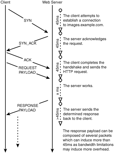
Why were the processes tied up for so long when serving all the content? Well, pinging www.example.com yields 90ms of latency from my workstation. TCP requires a three-way handshake, but we will only account for the first two phases because data can ride on the heels of the third phase making its latency contribution negligible. So, as shown in Figure 6.1, establishing the connection takes 90ms. Sending the request takes 45ms, and getting the response takes at least 45ms. Our www.example.com visit requires the loading of 59 individual pieces of content spread over seven connections yielding about eight requests per connection. On average, we see that each connection spent at minimum one handshake and eight request/responses summing to 900ms.
This constitutes 900ms out of the 4 seconds, so where did the rest go? Well, as is typical, my cable Internet connection, although good on average, only yielded about 500Kb/s (bits, not bytes). Our total page size was 167500 bytes (or 1340000 bits). That means 2.7 seconds were spent trying to fetch all those bits. Now this isn’t exact science as some of these seconds can and will overlap with the 900ms of latency shown in the previous paragraph, but you get the point—it took a while.
Now imagine dial-up users at 56Kb/s—the math is left as an exercise to the reader.
We’ve demonstrated that the Web is slow for most people. The goal is to speed it up, right? Yes, but that is more a secondary goal or side effect of accomplishing our real goal.
The real goal here is to cost effectively achieve a peak rate of 450,000 visitors per hour by making each visit take as few resources as possible, so that the same hardware (capital investment) can support many more visitors. This leads to scaling up (and down) the architecture more cost effectively.
Herein we will illustrate how to architect a web server solution that efficiently serves static content so that dynamic content web servers can continue to do their jobs. Only secondary is the goal of “accelerating” the end user’s experience.
More specifically, we want to segregate our traffic to allow for static content services to be hosted and even operated independently. This means that scaling image services up and down can be done orthogonally to scaling the dynamic services. Note that we want to allow for this, not require it.
The first step of accomplishing this goal, before we build out the architecture, is to support it from within the web application. This requires a change (usually minimal) in the application, or none at all if some foresight was used in its construction. To segregate the static and dynamic content on the www.example.com domain, we will migrate all the static content to a new base domain name: images.example.com. Although any web developer should be able to tackle this task blindfolded, I present a simple approach that can be taken with a grain of salt.
You could go through all your content and change IMG SRC tags to use nonrelative URLs of the form http://images.example.com/path/to/image.jpg. However, doing so will only leave you in the same position if you want to change back, change domain names, or switch to a third-party service such as Akamai or EarthCache.
Instead, you should create a method or function that can be used to dynamically generate static URLs. A short example in PHP:
Request.inc
<?
$default_http_static_base = 'http://images.example.com/';
function imgsrc($img) {
global $default_static_case;
return $http_static_base.$img;
}
?>
The php.ini file would be modified to "auto_prepend_file" Request.inc and in the PHP pages throughout the site, instead of placing images as <img src="/images/toplogo.jpg"> place them as <img src="<?= example_imgsrc('/images/toplogo.jpg')?>">. Using this methodology, to “scale down” and revert to the old method of a single instance for all traffic, simply change the $default_http_static_base back to "http://www.example.com/".
Now that we have all our static content pointing to images.example.com, let’s build a tuned cluster to support it.
The ultimate goal of this cluster is to serve static content more cost effectively than the main dynamic web servers can. Instead of being vague, let’s have a specific goal.
We want to build a static image serving cluster to handle the static content load from the peak hour of traffic to our www.example.com site. We’ve described peak traffic as 125 initial page loads per second and 500 subsequent page loads per second. Optimizing the architecture that serves the 625 dynamic pages per second will be touched on in later chapters. Here we will just try to make the infrastructure for static content delivery cost effective.
We need to do a bit of extrapolation to wind up with a usable number of peak static content requests per second. We can start with a clear upper bound by referring back to Table 6.1:
(125 initial visits / sec * 58 objects / initial visit) +
(500 subsequent visits / sec * 9 objects / subsequent visit) = 11750
objects/second
As discussed earlier, this is an upper bound because it does not account for two forms of caching:
-
The caching of static content by remote ISPs—In the United States, for example, America Online (aol.com) subscribers constitute more than 20% of online users of several major websites. When ISPs such as AOL deploy web caches, they can cause a dramatic decrease in static content requests. In the best case, we could see 20% less static traffic.
-
User browser caching—Many browsers aggressively cache static documents (even beyond the time desired by website owners). The previous numbers assume that the browser will cache images for the life of the session, but in truth that is a conservative speculation. Often images cached from prior days of web surfing may still reside in cache and can be utilized to make pages load faster. This also decreases the static request rate across the board.
The actual reduction factor due to these external factors is dependent on what forward caching solutions ISPs have implemented, and how many users are affected by those caches and the long-term client-side caches those users have.
We could spend a lot of time here building a test environment that empirically determines a reasonable cache-induced reduction factor, but that sort of experiment is out of the scope of this book and adds very little to the example at hand. So, although you should be aware that there will be a nonzero cache-induced reduction factor, we will simplify our situation and assume that it is zero. Note that this is conservative and errs on the side of increased capacity.
We are going to build this rip-roaring static cluster serving traffic. First we’ll approach the simplest of questions: How does the content get onto the machines in the first place?
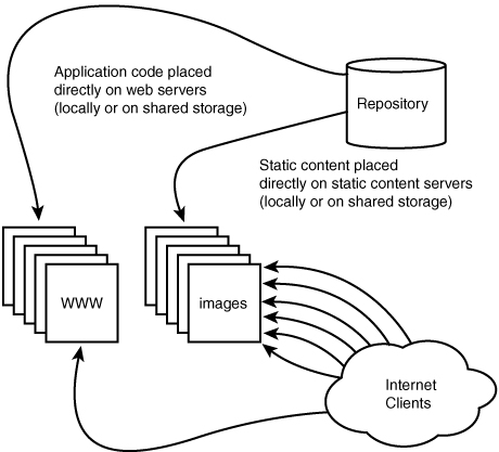
A priori placement is just a fancy way of saying that the files need to be hosted on each node before they can be served from that node as depicted in Figure 6.2. This is one of the oldest problems with running clusters of machines, solved a million times over and, luckily for us, simplified greatly due to the fact that we are serving cacheable static content.
Dynamic content typically performs some sort of business logic. As such, having one node execute the new version of code and another execute an older version spells disaster, specifically in multinode environments where each in the sequence of requests that compose a user’s session may be serviced by different nodes. Although it is possible to “stick” a user to a specific node in the cluster, we already discussed in Chapter 5, “Load Balancing and the Utter Confusion Surrounding It,” why this is a bad idea and should be avoided if possible.
Static content distribution, on the other hand, is a much simpler problem to address because we have already forfeited something quite important: control. To serve static content fast(er), we allow remote sites to cache objects. This means that we can’t change an object and expect clients to immediately know that their cached copies are no longer valid. This isn’t a problem logistically at all because new static objects are usually added and old ones removed because changing an object in-place is unreliable.
This means that no complicated semantics are necessary to maintain clusterwide consistency during the propagation of new content. Content is simply propagated and then available for use. Simply propagated... Hmmm...
The issue here is that the propagation of large sets of data can be challenging to accomplish in both a resource- and time-efficient manner. The “right” approach isn’t always the most efficient approach, at least from a resource utilization perspective. It is important to align the techniques used to distribute content to your application servers and static servers in a manner that reduces confusion. If developers or systems administrators have to use different policies or take different pitfalls into consideration when pushing static content as opposed to dynamic content, mistakes are bound to happen.
This means that if you push code by performing exports directly from your revision control system, it may be easier to propagate static content via the same mechanism. Although an export may not be as efficient as a differential transfer of content from a “master server,” only one mentality must be adopted—and remember: Humans confuse easily.
If no such infrastructure exists, we have several content distribution options.
Use a network file system. One copy of the content exists on a file server accessible by all web servers. The web servers mount this file system over IP and access the content directly. This is a popular solution in some environments, but poses a clear single point of failure because the clients cannot operate independently of the single file server. This approach also has certain deficiencies when used over a wide-area network.
AFS and CODA are “next-generation” network file systems. Both AFS and CODA allow for independent operation of the master file server by caching copies of accessed files locally. However, this technology is like implementing cache-on-demand on a different level in the application stack. Although these protocols are more friendly for wide areas, they still suffer from a variety of problems when operating in a disconnected manner.
This technique involves moving only the data that has changed from the content distribution point to the nodes in need. You are probably familiar with the freely available (and widely used) tool called rsync that implements this. Rsync provides a mechanism for synchronizing the content from a source to a destination by first determining the differences and then transferring only what is needed. This is extremely network efficient and sounds ideal. However, the servers in question are serving traffic from their disks and are heavily taxed by the request loads placed on them. Rsync sacrifices local resources to save on network resources by first performing relatively inexpensive checksums across all files and then comparing them with the remote checksums so that unnecessary data transfers can be avoided.
The “relatively inexpensive” checksums don’t seem so inexpensive when run on a highly utilized server. Plus, all our nodes need to sync from a master server, and, although rsync is only consuming marginal resources on each of the N nodes, it is consuming N times as many resources on the master server.
Hence, the world needs a network-efficient, resource-efficient 1 to N content distribution system with rsync’s ease of use. Consider this a call to arms.
Directly exporting from revision control, assuming that your content is stored in some revision control system (as it certainly should be), has tremendous advantages. All the uses for revision control of code directly apply to static content: understanding change sets, backing out changes, and analyzing differences between tags or dates.
Most systems administrators are familiar with some version of revision control, and all developers should be fluent. This means that revision control is not only philosophically compatible with the internal control of static content but also is familiar, intuitive, and usable as well.
With so much praise, why isn’t this approach used by everyone? The answer is efficiency. CVS is the most popular revision control system around due to its licensing and availability. CVS suffers from terrible tag times, and exports on large trees can be quite painful. Even with commercial tools and newer open free tools such as Subversion, the efficiency of a large checkout is, well, inefficient.
Most well-controlled setups implement exports from revision control on their master server and use a tool such as rsync to distribute that content out to the nodes responsible for serving that traffic, or opt for a pure cache-on-demand system.
Cache-on-demand uses a different strategy to propagate information to a second (or third, or fourth) tier. A variety of commercial solutions are available that you simply “plug in” in front of your website, and it runs faster. These solutions typically deploy a web proxy in reverse cache mode.
Web caches were originally deployed around the Internet in an attempt to minimize bandwidth usage and latency by caching commonly accessed content closer to a set of users. However, the technologies were designed with high throughput and high concurrency in mind, and most of the technologies tend to outperform general-purpose web servers. As such, a web cache can be deployed in front of a busy website to accomplish two things:
-
Decrease the traffic directed at the general web servers by serving some of the previously seen content from its own cache.
-
Reduce the amount of time the general purpose web server spends negotiating and tearing down TCP connections and sending data to clients by requiring the general purpose web server to talk over low-latency, high-throughput connections. The web cache is responsible for expensive client TCP session handling and spoon-feeding data back to clients connected via low-throughput networks.
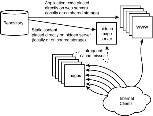
Web caches handle client requests directly by serving the content from a local cache. If the content does not exist in the local cache, the server requests the content from the “authoritative” source once and places the resulting content in the local cache so that subsequent requests for that data do not require referencing the “authoritative” source. This architecture is depicted in Figure 6.3.
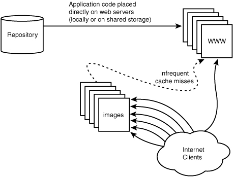
Web caches that operate in this reverse proxying fashion are often called web accelerators. Apache with mod_proxy and Squid are two popular, widely adopted caching solutions commonly deployed in this configuration. Figure 6.3 shows a configuration in which the authoritative source is the main website. We can remove this marginal load from the dynamic servers by placing the content a priori on a single static content server that is hidden from the public as seen in Figure 6.4.
Let’s continue our route of using free software, as Apache is already at the core of our architecture. Apache 1.3.x with a relatively vanilla install clocks in at about 800 requests per second on our server. Our goal is to service 11,750 requests per second, and we don’t to not exceed 70% capacity, which leaves us with a need for (11,750/70%)/800 = 20 servers. Each server here is capable of pushing about 16MB/s. Although commodity servers such as this have a list price of around $2,000 each, totaling at a reasonable $40,000, 20 servers for static images seems, well, less than satisfying.
Because we are serving static traffic, several other web server technologies could be used with little or no effort, instead of Apache. A quick download and compile of thttpd yields better results at approximately 3500 requests per second on the same server pushing about 70MB/s. Repeating the previous server calculations with our new metrics, we now need five servers—(11,750/70%)/3,500 rounded up.
A valuable feature exists in Apache and is notably absent in thttpd. This is reverse-proxy (web cache) support. This feature is useful because it allows you to build a cluster with a different strategy and adds elegance and simplicity to the overall solution. thttpd requires a priori placement of content, whereas Apache can use both a priori placement of content and cache-on-demand via the mod_proxy module. As we have seen, it takes 20 servers running Apache to meet the capacity requirements of our project, so let’s find a higher performance caching architecture.
Apache is slower than thttpd in this particular environment for several reasons:
-
It is more flexible, extensible, and standard.
-
It is more complicated and multipurposed.
-
It uses an architectural model that allocates more resources to each individual connection.
So, logically, we want to find a web server capable of proxying and caching data that is single-purposed, simple, and extremely efficient on a per-connection basis. Some research leads us to Squid (www.squid-cache.org). Architecturally, it is similar to thttpd, but single-purposed to be a web cache.
Cache-on-demand systems are inherently less efficient than direct-serve content servers because extra efforts must be made to acquire items that are requested but not yet in the cache and to ensure that data served from cache is still valid. However, a quick test of Squid is a good indication as to whether such a performance degradation is acceptable.
By installing Squid in http acceleration mode, we can benchmark on the same hardware around 2,800 requests per second. This is 20% slower. However, we see that this only increases our single location requirements to (11,750/70%)/2,800 and thus six servers.
Several commercial products boast higher performance than Squid or Apache. The adoption of any such device is really up to the preference of the operations group. Growing a solution based on open-sourced technologies tends to have clear technical and financial advantages for geographically distributed sites because costs multiply rapidly when commercial technologies are used in these situations. This is basically the same argument that was made in Chapter 4, “High Availability. HA! No Downtime?!.” Adding a high performance appliance to a setup is often an easy way to accomplish a goal, just remember you need two for high availability. Although this may make good sense at a single highly trafficked location, if the site were to want a presence at four geographically unique locations, you have just committed to six more of these appliances (two at each site). Whether that is right is a decision you need to make for yourself.
Six servers are better than 20 for more reasons than capital hardware costs. A smaller cluster is easier and cheaper to manage, and, as discussed in previous chapters, it simplifies troubleshooting problems. Because this cluster serves only the simplest of content, we are not impressed with the extra added features of Apache and its modules, and do not find them to be a compelling reason to choose it over a smaller, simpler, and faster solution for our project at hand.
The architecture supporting the static content for www.example.com must maintain the same (or stricter) availability requirements as the dynamic systems because it is a necessary part of the overall service. Our peak traffic is expected to be 11,750 requests per second, so we should be able to satisfy that metric with four servers, leaving us two for truly unexpected traffic surges and hardware failures.
This means that we must build a two-fault tolerant system that has remedial balancing of traffic. Multiple DNS RR A records should be sufficient for distributing incoming requests naively across the six machines, leaving an IP availability issue that can easily be solved by Wackamole.
For this cluster, we will use FreeBSD 4.9. Why? Simply because. This is not because FreeBSD is better than Linux is better than Solaris is better the Joe’s OS, and so on. Honestly, any of these Unix and Unix-like systems should work like a charm. So, why do we choose FreeBSD as an example?
-
It is a popular platform on which to run Squid, so community support for Squid on this platform will likely be of a higher caliber. Additionally, Squid supports the kqueue event system on FreeBSD allowing it to boast higher concurrency at lower CPU utilization than some other platforms.
-
Wackamole supports FreeBSD more thoroughly than Solaris or Linux. More tested installations means less likelihood of failure.
-
For the sake of an example in literature, the whole “which Linux distribution” religious war can be avoided.
We install six commodity servers with a FreeBSD 4.9 default install and assign each its public management IP address, 192.0.2.11 through 192.0.2.16, and name them image-0-1 through image-0-6, respectively.
Appropriate firewall rules should be set to protect these machines. Although this is outside the scope of this book, we can discuss the traffic we expect to originate from and terminate at each box.
-
Inbound port 80 TCP and the associated established TCP session (for web serving)
-
Inbound port 22 TCP and the associated established TCP session (ssh for administration)
-
Outbound port 53 UDP and the corresponding responses (for DNS lookups)
-
Inbound/Outbound Port 3777 UDP/TCP and 3778 UDP (to peer machines for Spread needed by Wackamole)
It is important to note that the six IP addresses above the management IPs and all client-originating web traffic will arrive to the IP published through DNS for this service.
Wackamole is a product from the Center for Networking and Distributed Systems at the Johns Hopkins University and is an integral part of the Backhand Project (www.backhand.org).
Wackamole’s goal is to leverage the powerful semantics of group communication (Spread specifically) to drive a deterministic responsibility algorithm to manage IP address assignment over a cluster of machines. The technology differs from other IP failover solutions in that it can flexibly support both traditional active-passive configuration, as well as power multi-machine clusters where all nodes are active.
In Chapter 4, we briefly discussed the technical aspects of Wackamole; now we can discuss why it is the “right” solution for this problem.
There are several reasons for choosing Wackamole aside from my clearly biased preference toward the solution. The alternative solutions require placing a machine or device in front of this cluster of machines. Although this works well from a technical standpoint, its cost-efficiency is somewhat lacking. As discussed in Chapter 4, to meet any sort of high availability requirements, the high-availability and load-balancing (HA/LB) device needs to be one of a failover pair.
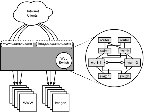
You also might argue that you already have a hardware load balancer in place for the dynamic content of the site, and you can simply use those unsaturated resources as shown in Figure 6.5. This is a good argument and a good approach. You have already swallowed the costs of owning and managing the solution, so it does not incur additional costs while the management of a Wackamole-based solution does. However, another reason has not been mentioned yet—growth.
The last section of this chapter discusses how to split the solution geographically to handle higher load and faster load times for users. Clearly, if this architecture is to be replicated twice over, the costs of two HA/LB content switches twice over will dramatically increase the price and complexity of the solution.
Although it is arguable that Wackamole is not the right solution for a single site if an HA/LB content-switching solution is already deployed at that site, it will become clear that as the architecture scales horizontally, it is a cost-effective and appropriate technology.
Wackamole, first and foremost, requires Spread. Appendix A, “Appendix,” details the configuration and provides other tips and tricks to running Spread in production. For this installation, we will configure Spread to run listening to port 3777.
Wackamole is part of the Backhand project and can be obtained at www.backhand.org. Compiling Wackamole is simple with a typical ./configure; make; make install. For cleanliness (and personal preference), we’ll keep all our core service software in/opt. We issue the following commands for our install:
Installed as it is, we want a configuration that achieves the topology portrayed in Figure 6.6. This means that the six machines should manage the six IP addresses published through DNS. Now the simplicity of peer-based failover shines.
Which machine should get which IP address? As a part of the philosophy of peer-based HA, that question is better left up to the implementation itself. Wackamole should simply be told to manage the group of IP addresses by creating a wackamole.conf file as follows:
Spread = 3777
Group = wack1
SpreadRetryInterval = 5s
Control = /var/run/wack.it
Prefer None
VirtualInterfaces {
{ fxp0:192.0.2.21/32 }
{ fxp0:192.0.2.22/32 }
{ fxp0:192.0.2.23/32 }
{ fxp0:192.0.2.24/32 }
{ fxp0:192.0.2.25/32 }
{ fxp0:192.0.2.26/32 }
}
Arp-Cache = 90s
mature = 5s
Notify {
# Let's notify our router
fxp0:192.0.2.1/32
# And everyone we've been speaking with
arp-cache
}
Let’s walk through this configuration file step-by-step before we see it in action:
-
Spread—Connects to the Spread daemon running on port 3777. -
Group—All Wackamole instances running this configuration file will converse over a Spread group namedwack1. -
SpreadRetryInterval—If Spread were to crash or otherwise become unavailable, Wackamole should attempt to reconnect every 5 seconds. -
Control—Wackamole should listen on the file /var/run/wack.it for commands from the administrative program wackatrl. -
Prefer—Instructs Wackamole that no artificial preferences exist toward any one IP. In other words, all the Wackamoles should collectively decide which servers will be responsible for which IP addresses. -
VirtualInterfaces—Lists the IP addresses that the group of servers will be responsible for. These are the IP addresses published through DNS for images.example.com that will “always be up” assuming that at least one machine running Wackamole is alive and well. -
Arp-Cache—Instructs each instance to sample the local machine’s ARP cache and share it with the other cluster members. The ARP cache contains the IP address to Ethernet MAC address mapping that is used by the operating system’s network stack to communicate. It contains every IP address that a machine has been communicating with “recently.” If machine A fails, and B is aware of the contents of A’s ARP cache, B can inform all the necessary machines that have been communicating with A that the MAC addresses for the services they need have changed. -
Mature—To reduce “flapping,” 5 seconds are allowed to pass before a new member is eligible to assume responsibility for any of the virtual interfaces listed. -
Notify—When Wackamole assumes responsibility for an IP address, it informs its default route at 192.0.2.1 and every IP address in the cluster’s collective ARP cache. This is an effort to bring quick awareness of the change to any machines that have been using the services of that IP address.
Now that Wackamole is installed, let’s crank it up and see whether it works. First we will bring up Spread on all the machines (it should be in the default start scripts already) and test it as described in Appendix A. Next, we start Wackamole on image-0-1:
root@image-0-1# /usr/local/sbin/wackamole
root@image-0-1# /usr/local/sbin/wackatrl –l
Owner: 192.0.2.11
* fxp0:192.0.2.21/32
* fxp0:192.0.2.22/32
* fxp0:192.0.2.23/32
* fxp0:192.0.2.24/32
* fxp0:192.0.2.25/32
* fxp0:192.0.2.26/32
root@image-0-1# ifconfig fxp0
fxp0: flags=8843<UP,BROADCAST,RUNNING,SIMPLEX,MULTICAST> mtu 1500
inet 192.0.2.11 netmask 0xffffff00 broadcast 192.0.2.255
inet6 fe80::202:b3ff:fe3a:2e97%fxp0 prefixlen 64 scopeid 0x1
inet 192.0.2.21 netmask 0xffffffff broadcast 192.0.2.21
inet 192.0.2.22 netmask 0xffffffff broadcast 192.0.2.22
inet 192.0.2.23 netmask 0xffffffff broadcast 192.0.2.23
inet 192.0.2.24 netmask 0xffffffff broadcast 192.0.2.24
inet 192.0.2.25 netmask 0xffffffff broadcast 192.0.2.25
inet 192.0.2.26 netmask 0xffffffff broadcast 192.0.2.26
ether 00:02:b3:3a:2e:97
media: Ethernet autoselect (100baseTX <full-duplex>)
status: active
So far, so good. Let’s make sure that it works. From another location, we should ping all six of the virtual IP addresses to ensure that each is reachable. After successfully passing ICMP packets to these IP addresses, the router or firewall through which image-0-1 passes packets will have learned that all six IP addresses can be found at the Ethernet address 00:02:b3:3a:2e:97.
Now we bring up image-0-2:
root@image-0-2# /usr/local/sbin/wackamole
root@image-0-2# /usr/local/sbin/wackatrl –l
Owner: 192.0.2.11
* fxp0:192.0.2.21/32
* fxp0:192.0.2.22/32
* fxp0:192.0.2.23/32
Owner: 192.0.2.12
* fxp0:192.0.2.24/32
* fxp0:192.0.2.25/32
* fxp0:192.0.2.26/32
root@image-0-2# ifconfig fxp0
fxp0: flags=8843<UP,BROADCAST,RUNNING,SIMPLEX,MULTICAST> mtu 1500
inet 192.0.2.12 netmask 0xffffff00 broadcast 192.0.2.255
inet6 fe80::202:b3ff:fe3a:2f97%fxp0 prefixlen 64 scopeid 0x1
inet 192.0.2.24 netmask 0xffffffff broadcast 192.0.2.24
inet 192.0.2.25 netmask 0xffffffff broadcast 192.0.2.25
inet 192.0.2.26 netmask 0xffffffff broadcast 192.0.2.26
ether 00:02:b3:3a:2f:97
media: Ethernet autoselect (100baseTX <full-duplex>)
status: active
Everything looks correct, but we should make sure that image-0-1 sees the same thing. Because the output of wackatrl –l will certainly be the same, ifconfig is the true tool to make sure everything is the same. Subsequent to bringing image-0-2’s Wackamole instance up, we see the appropriate message in /var/log/message, and ifconfig shows that the three complementary IP addresses are assigned to image-0-1.
root@image-0-1# tail /var/log/message | grep wackamole
image-0-1 wackamole[201]: DOWN: fxp0:192.0.2.24/255.255.255.255
image-0-1 wackamole[201]: DOWN: fxp0:192.0.2.25/255.255.255.255
image-0-1 wackamole[201]: DOWN: fxp0:192.0.2.26/255.255.255.255
root@image-0-1# ifconfig fxp0
fxp0: flags=8843<UP,BROADCAST,RUNNING,SIMPLEX,MULTICAST> mtu 1500
inet 192.0.2.11 netmask 0xffffff00 broadcast 192.0.2.255
inet6 fe80::202:b3ff:fe3a:2e97%fxp0 prefixlen 64 scopeid 0x1
inet 192.0.2.21 netmask 0xffffffff broadcast 192.0.2.21
inet 192.0.2.22 netmask 0xffffffff broadcast 192.0.2.22
inet 192.0.2.23 netmask 0xffffffff broadcast 192.0.2.23
ether 00:02:b3:3a:2e:97
media: Ethernet autoselect (100baseTX <full-duplex>)
status: active
Although the local configuration on each server looks sound, there is more to this than meets the eye. The traffic from other networks is being delivered to and from this one server through a router, and that router has an ARP cache. If the ARP cache was not updated, the router will continue to send packets to 192.0.2.24, 192.0.2.25, and 192.0.2.26 to image-0-1. Although we can be clever and send ICMP packets to each IP address and use a packet analyzer such as tcpdump or ethereal to determine whether the ICMP packets are indeed being delivered to the correct machine, there is a simpler and more appropriate method of testing this—turn off image-0-1.
Wackamole employs a technique called ARP spoofing to update the ARP cache of fellow machines on the local Ethernet segment. Machines use their ARP cache to label IP packet frames for delivery to their destination on the local subnet. When two machines on the same Ethernet segment want to communicate over IP, they each must ascertain the Ethernet hardware address (MAC address) of the other. This is accomplished by sending an ARP request asking what MAC address is hosting the IP address in question. This request is followed by a response that informs the curious party with the IP address and MAC address. The crux of the problem is that this result is cached to make IP communications efficient.
After we yank the power cord from the wall, we should see image-0-2 assume responsibility for all the IP addresses in the Wackamole configuration. Now a ping test will determine whether Wackamole’s attempts to freshen the router’s ARP cache via unsolicited ARP responses was successful.
If pings are unsuccessful and suddenly start to work after manually flushing the ARP cache on our router, we are unfortunate and have a router that does not allow ARP spoofing. The only device I am aware of that acts in this fashion is a Cisco PIX firewall, but I am sure there are others lingering out there to bite us when we least expect it.
If a server is communicating over IP with the local router, that router will inevitably have the server’s MAC address associated with that server’s IP address in its ARP cache. However, if that server were to crash and another machine was to assume the responsibilities of one of the IP addresses previously serviced by the crashed machine, the server will have the incorrect MAC address cached. Additionally, it will not know that it needs to re-ARP for that IP. So, Wackamole will send ARP response packets (also known as unsolicited or gratuitous ARPing) to various machines on the local Ethernet segment if an IP address is juggled from one server to another.
Assuming that all has gone well, our cluster is ready for some serious uptime. After bringing up all six Wackamole instances, we will see the following output from wackatrl –l.
root@image-0-2# /usr/local/sbin/wackatrl –l
Owner: 192.0.2.11
* fxp0:192.0.2.21/32
Owner: 192.0.2.12
* fxp0:192.0.2.22/32
Owner: 192.0.2.13
* fxp0:192.0.2.23/32
Owner: 192.0.2.14
* fxp0:192.0.2.24/32
Owner: 192.0.2.15
* fxp0:192.0.2.25/32
Owner: 192.0.2.16
* fxp0:192.0.2.26/32
Now, even if five of these machines fail, all six virtual IP addresses will be publicly accessible and serving whatever services necessary. Granted, our previous calculations let us know that one machine would never be capable of coping with the peak traffic load, but we still should be able to have two of them offline (unexpectedly or otherwise) and be able to handle peak load.
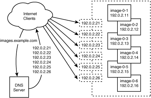
The next step is to advertise these six IP addresses via DNS so that people visiting images.example.com will arrive at our servers.
The DNS RR records for this service should look as follows:
$ORIGIN example.com.
images 900 IN A 192.0.1.21
900 IN A 192.0.1.22
900 IN A 192.0.1.23
900 IN A 192.0.1.24
900 IN A 192.0.1.25
900 IN A 192.0.1.26
This sample bind excerpt advertises the six listed IP addresses for the name images.example.com, and clients should “rotate” through these IP addresses. Clients, in this context, are not actually end users but rather the caching name server closest to the client. Each name server is responsible for cycling the order of the records it presents from response to response. So each new query for images.example.com results in a list of IP addresses in a new order. Typically, web browsers tend to use the name service resolution provided by the host machine that they run on, and most hosts choose the first DNS RR record when several are presented. That means different clients accessing the same name server will contact different IPs, and there will be a general distribution across all the advertised IPs.
The balancing will not be even, but you should see roughly the same number of requests per second across each of the IP addresses. For example, in our production reference implementation, we see an average 30% deviation from machine to machine on a second-to-second basis, and less than 3% deviation from minute to minute. So, although the balancing is not perfect, it is entirely sufficient.
Now that we have six servers clustered together, we need to set up a high-performance web serving platform to meet our needs—a peak demand of 11,750 requests per second.
Installing Squid is fairly straightforward with a familiar ./configure; make; make install. However, configuring it can be complicated.
The main squid.conf file should be modified to make the Squid instance act as an HTTP accelerator only for images.example.com.
http_port 80 accel vhost vport=80 defaultsite=images.example.com
acl all src 0.0.0.0/0.0.0.0
acl manager proto cache_object
acl localhost src 127.0.0.1/255.255.255.255
acl to_localhost dst 127.0.0.0/8
acl Safe_ports port 80
acl CONNECT method CONNECT
http_access allow manager localhost
http_access deny manager
http_access deny !Safe_ports
http_access deny to_localhost
http_access deny CONNECT
http_access allow all
acl acceld dstdomain images.example.com
always_direct allow acceld
This allows requests to this cache from anywhere but only pulls content to satisfy those requests of images.example.com. images.example.com should be added to the local /etc/hosts file to be the published IP of www.example.com. This configuration achieves the content placement approach shown previously in Figure 6.3.
Our news site is now cranking along, serving static content to visitors. The solution we have built works well. Visitors from all around the world visit www.example.com and fetch images from our small and efficient cluster. As with any good system, however, there is always room for improvement.
Of course, nothing initiates improvements like a change in requirements. The site has been performing adequately from a technical point of view, but example.com has been overperforming on the business side—we all should be so lucky. We have been tasked by management to increase the capacity of the whole system by a factor of four to meet expected demand.
Scaling the systems downward that we built before could not be easier. Unplugging, moving from the cabinets, and liquidating some of the static servers would have done the trick—no administration required. However, scaling up requires some work. The goal is to have a technology base that is sound and efficient enough to be grown without core change. We will see that we have accomplished this.
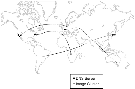
The one aspect of image serving that is deficient, aside from our sudden lack of capacity, is our ability to capitalize on user proximity. Essentially, everyone in the world is visiting our site in San Jose, California, in the United States. Although this is probably great for people on the West Coast of the United States, it leaves a lot to be desired for visitors from the United Kingdom, the rest of Europe, Asia, Africa, and even the East Coast of the United States.
Figure 6.7 shows this configuration from a global perspective. Earlier, we analyzed the resource costs of latency and found that the resources idly tied up by the latency in a TCP connection to a web server is second only to that incurred by low-bandwidth connections. Although a single intercontinental or cross-continental TCP request for a single object may not be painfully slow, six connections for 58 objects certainly is. By providing a static cluster closer to the end user, we intrinsically reduce latency and have a good chance of increasing throughput by reducing the number of possibly congested networks through which packets flow.
Ideally, we want to place static content servers in a position to serve the bulk of our visitors with low latency. Upon further investigation into the business issues that sparked this needed capacity, we find that the reason is a doubling of traffic in the United States and good penetration into the European and Asian markets.
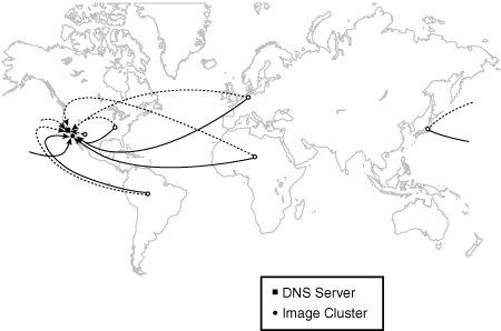
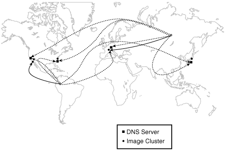
With this in mind, a placement in Japan, Germany, New York, and San Jose would be reasonably close to the vast majority of our intended audience. However, special care should be taken. The system must be designed correctly, or what we hope to accomplish will backfire. We want users to visit the content distribution point closest to them. However, the architecture, in its raw form, affords the opportunity to have users visit a distribution point that is very far away, as shown in Figure 6.8.
Clearly this type of introduced inefficiency is something to avoid. So, how do we make sure that users in Europe visit our content distribution point in Europe and likewise for other countries and locations? We’ll take a very short stab at answering this question and then talk about why it is the wrong question to ask.
To have users in Europe visit our installation in Germany, we can determine where in the world the user is and then direct them to a differently named image cluster. For example, Germany could be images.de.example.com, and Japan could be images.jp.example.com. To determine “where” the user is, there are two basic options. The first is to ask the user where she is and trust her response. This is sometimes used to solve legal issues when content must differ from viewer to viewer, but we do not have that issue. The second is to guess the location from the client’s IP address. Unfortunately, both these methods have a high probability of being inaccurate.
We have gone astray from our goal with a subtly incorrect assumption. Our goal was to reduce latency and possibly increase throughput by moving the origin of content closer to the user. So far, so good. Then we conjectured about how we should determine whether a user is geographically closer to one location or another. Somehow, that “geographical” qualifier slipped in there, likely because people prefer to think spatially. The truth of the matter is that you don’t care where in the world (literally) the user is, just where on the Internet the user is. The proximity we should be attempting to capitalize on is the user’s proximity on the network.
The problem has been more clearly defined and is now feasible to solve using some network-based techniques.
The DNS Round-Trip Times method relies on each local name server tracking the round-trip time of packets as it performs recursive name service resolution. Over time, the local recursive name server will favor authoritative servers with the lowest latency. This “optimization strategy” results in resolution being performed against the authoritative DNS server “closest” to the client’s name server with respect to the network—or so the theory goes.
Rephrased and simplified a bit, the client attempts to resolve images.example.com from each authoritative name server, eventually settling on the name server with the quickest responses.
So, all we need to do is put a publicized, authoritative name server for images.example.com alongside each image cluster at our four locations. Each name server will serve the IP addresses of the onsite image servers. As shown in Figure 6.9, the name server in Germany serves the IP addresses for the cache servers in Germany, the name server in Japan serves the IP addresses for the cache servers in Japan, and so on.
This method is easy to implement and requires no special infrastructure, but it suffers from some rather serious shortcomings. The most obvious is that the algorithm calls for the “eventual” convergence on the closest name server, and until each client’s local name server converges, you have misdirection. Additionally, sudden changes in network topology, such as a collapsed route or the peering relationship between two autonomous systems (ASs) changing, will cause the answer we spent so much time reaching to be suboptimal. The Internet is a rapidly changing place—a sea of endpoints. Point A will most likely always be able to communicate with point B, but the routers and networks those packets traverse can change at any moment.
There is another method to find the closest server on the network that copes well with the nature of the Internet by leveraging the fundamentals of efficient network routing (that is, delivering packets to an IP address over the shortest path).
By giving two different servers on the Internet the same IP address and requesting the networks to which we are attached to announce the routes to those IP addresses (as is normally done), we employ the technique now called Anycast.
The tricky part about using Anycast is that, at any moment in time, routes can change. This means that the next packet sent to that IP address might very well find its way to a different host. What does this mean in terms of IP? Given that all DNS traffic and web serving happens over IP, this is an important question.
If host image-2-1.example.com in Germany and image-3-1.example.com in Japan share the same IP address, the following scenario is possible. A client attempts to establish a TCP connection to images.example.com. The client first resolves the name to an IP address to which the client sends a SYN packet (sent as the first step in establishing a TCP connection) that finds its way to image-2-1.example.com (in Germany). The ACK packet is sent back to the client, and the client then sends back the first data packet containing the http request. All is well until now. Then a route flaps somewhere on the Internet, and the closest path from that client to the destination IP address now delivers packets to image-3-1.example.com (in Japan).
image-2-1 returns a data packet to the client, and it gets there because the shortest path from image-2-1 to the client does not lead the packet astray (there is only one machine on the Internet with that client’s IP address). However, when the client responds to that packet, it goes to Japan (the new shortest path back to the server IP). This is where things go sour. When the packet arrives at image-3-1, it is part of a preexisting TCP session with image-2-1 of which image-3-1 knows nothing. The only reasonable response to this is to send a TCP RST packet, which aborts the TCP session, and that’s no good at all.
So, what good is Anycast? Well, we’ve demonstrated the shortcomings with respect to TCP. But these shortcomings hinge on the connectedness of that transport protocol. UDP, on the other hand, is a connectionless protocol. Services such as DNS typically only require a single request and response UDP packet to accomplish a task. So, where does this leave us?
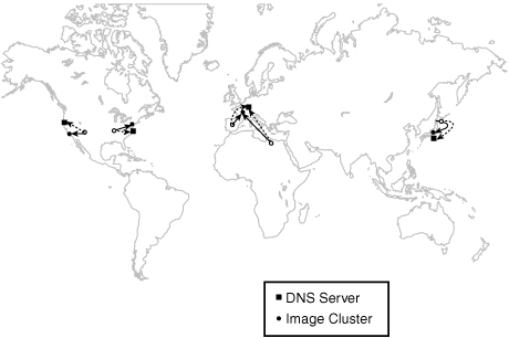
We know that each node in each image cluster needs a unique IP address to avoid the problem described previously. If we place DNS servers next to each image cluster and all DNS servers share the same IP address (via Anycast) and each DNS server offers the IP addresses of the image cluster nodes nearest to it, we achieve our proximity objectives. Figure 6.10 shows our globally distributed system based on Anycast.
Anycast ensures that a client’s DNS requests will be answered by the DNS server closest to him on the network. Because the DNS server handed back the IP addresses associated with the image server to which it is adjacent, we know that (as the DNS request traversed the Internet) this image cluster was the closest to the client. That’s pretty powerful mojo.
We now know how to construct a static content distribution network capable of servicing a peak load of 47,000 queries per second (assuming full utilization on each cluster). More importantly, we have accomplished the following goals:
-
Build a static content acceleration server to make our news site faster.
-
Reduce the latency and potentially increase the throughput for most users’ requests to the site.
-
Build something from scratch that is easy to maintain, inexpensive to build, and inexpensive to operate in the long run.
Our final architecture has four identical cluster installs that are globally and strategically placed.
-
Each cluster is completely functional and standalone. Six inexpensive commodity machines running Wackamole for IP failover provide high availability and high performance.
-
The architecture runs Squid and acts as a cache-on-demand system that needs no out-of-band content synchronization.
-
DNS servers using Anycast ensure that clients are delivered to the most network-appropriate cluster.
Earlier a statement was made: “It will become clear that as the architecture scales horizontally, it is a cost-effective and appropriate technology.” Let’s look at this a bit more to better understand the drastic savings resulting from this architecture choice over a classic “white-paper” approach.
Figure 6.5 shows what the architecture would look like if the image cluster was fronted by the same web switch that drives the load-balancing for the dynamic content cluster. The “web switch” in that diagram is really two routers, four wiring-closet switches, and two web switches. When we presented the architecture depicted in Figure 6.7 in context, it was reasonable because that infrastructure was already there to support the dynamic application, so there was no investment to be made. However, by placing the image clusters at three other locations in the world, we would now need that same “web switch” in front of each.
In all fairness, we can’t just ignore all that hardware. We will need portions of it in the new architecture—namely two routers and two switches at each location for high availability. But immediately we see that we can avoid purchasing six wiring-closet switches and six web switches. Let’s put some dollars on that.
Web switches capable of actually load-balancing more than 200Mbs of traffic carry a pretty price tag—often more than $50,000 each. Wiring-closet switches often run around $5,000 each. That adds up to $625,000. Well worth it if you ask me.