
Radar technology: radio frequency, interferometric, millimeter wave and terahertz sensors for assessing and monitoring civil infrastructures
D. Huston, University of Vermont, USA
D. Busuioc, DB Consulting, USA
Abstract:
Radar and millimeter wave methods provide a means of remote and noncontacting examination of structures through controlled electromagnetic (EM) interactions. Metallic and nonmetallic structures reflect and scatter EM waves impinging at the outer surfaces. Nonmetallic, i.e., dielectric, materials allow for EM waves to penetrate the surface, and scatter or reflect off of subsurface objects and features. Actively measuring surface and subsurface reflectivity and scattering by the controlled launching and receiving of EM waves provides information that when suitably processed can indicate surface and subsurface feature geometry, material properties, and overall structural condition. These active EM technical tests are often called ‘Ground Penetrating Radar’ for EM wave frequencies less than about 10 GHz and ‘Millimeter Wave’ methods for those at higher frequencies. This chapter describes the range of uses, operating principles, signal processing, and data interpretation for these methods.
Key words
electromagnetic; ground penetrating radar; radar; millimeter wave; dielectric; concrete; corrosion
8.1 Introduction
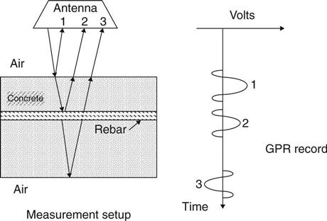
Radar-based sensors use radio frequency (RF) and higher electromagnetic (EM) field disturbances to identify, locate, and assess structures and materials. Civil engineering applications include probing subsurface conditions in concrete, asphalt, and masonry for cracks, delaminations, and corrosion; determining the presence of water, ice, or other contaminants on surfaces; detecting corrosion under painted surfaces; imaging objects through walls; and overall geometric structural shape assessment. An important feature of radar sensing is that the EM field disturbances act both as probes for measurement and as signal transmitters. Figure 8.1 shows a typical sensing system configuration that generates, measures, and analyzes EM fields.

Many of these instruments are known as ground penetrating radars (GPR). Interferometric, millimeter wave, and/or terahertz sensors are more accurate terms for some of these systems.
Radar and millimeter wave sensors have several advantages:
1. An ability to sense remote and subsurface conditions with a convenience that is difficult to match with other sensors.
2. An underlying sensing mechanism that operates at the speed of light. Measurement throughput can be quite fast.
3. The energy in the EM fields is generally small, inherently safe, and nondestructive.
4. The performance versus cost of the sensor systems continues to improve with ongoing developments in hardware, software, and testing protocols.
5. The instrument operators need only a modest level of training.
1. EM waves cannot penetrate all materials. Conductors reflect EM waves. Lossy dielectrics quickly absorb and attenuate waves. Nonhomogeneous materials scatter EM waves and reduce the strength of return signals.
2. Longer wavelengths and lower frequency waves generally tend to penetrate more deeply into dielectric materials, but at a cost of reduced spatial resolution.
3. Complicated signal processing techniques are often required.
4. Many data sets routinely require highly trained experts for interpretation.
5. The instruments tend to be relatively expensive and complicated.
6. Government agencies regulate the levels of radiated EM emissions. This constrains achievable penetration depths and other performance parameters.
8.2 Brief history of ground penetrating radar (GPR) systems
GPRs transmit high-frequency EM waves out through specialized antennas. The waves project onto, and often penetrate into, the surfaces of solids. A portion of the waves reflects back to a receiver antenna. The arrival time, shape, and amplitude of the return wave relates to the location, variation, and nature of dielectric properties in the material (air/asphalt or asphalt/concrete, reinforcing steel, etc.). Figure 8.2 shows how an EM wave reflects off of features inside a steel reinforced concrete bridge deck. Capturing, processing, and displaying the reflected wave signals illustrates the subsurface dielectric properties, which often correlate with underlying material properties of interest.
The roots of GPR technology lie in the development of EM field theories by some of the prominent physicists of the nineteenth century (Ampere, Heaviside, Henry, Hertz, Maxwell, Lorenz) and through the first half of the twentieth century with the development of radio transmission systems (Annan, 2002). The 1940s, with the Second World War, gave rise to the rapid development of radar systems, primarily for the location of airplanes and ships. The first noted use of radar to probe subsurface conditions was in 1956 with the detection of water table depths by El Said in 1956 (El Said, 1956). Geological and archeological applications appeared in the 1970s, especially for materials with low losses, such as coal and salt (Holser et al., 1972; Cook, 1973; Thierbach, 1974). Commercial GPR systems became available following the 1970 formation of Geophysical Survey System, Inc. in Salem, NH (GSSI) (Morey, 1974). An early civil engineering application was geological evaluations of Alaska pipeline routes by Olhoeft (Olhoeft, 1975).
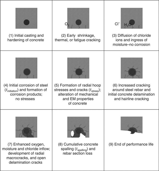
The need for a convenient nondestructive tool for assessing steel reinforced concrete bridge decks motivated much of the development of GPR for structural engineering. Corrosion of steel reinforcing bars is a major maintenance problem. Many of the problems are progressive damage processes that start with the combined application of deicing salts, harsh environmental and loading conditions, and end with the disintegration of the roadway. Normally, the alkaline nature of concrete forms a passivating layer that protects embedded steel from corrosion. Chlorides, water, and oxygen can break the passivation layer and initiate a complicated multiyear process that eventually renders the deck unserviceable (Fig. 8.3). Similar processes occur in other concrete structural elements. Early detection with instruments, such as GPR, can enable early and low cost intervention.
Some of the notable structural engineering studies of GPR in the early 1980s include that of Steinway et al. (1981), Ulriksen (1982), Alongi et al. (1982), Manning and Holt (1984), Chung et al. (1984), and Clemena and Joyce (1984). The indication was that GPR instruments could detect layers in asphalt-overlaid concrete and bare concrete bridge decks. The presence of chlorides increased asphalt reflectivity. Good concrete exhibited a ‘smoother’ waveform than distressed concrete. Maser (1989) found a positive correlation between the total deterioration observed on asphalt-overlaid bridge decks and the high values of the dielectric constant of the concrete measured immediately below the asphalt layer. Based on the observation that the amplitudes of the reflections from subsurface steel reinforcing bars drop off with increased chloride content, and possibly with delaminations, an attempt to standardize resulted in the provisional specification AASHTO TP36–93 (1993). This specification was not widely adopted, but the underlying concept remains relevant today.
Starting in the late 1980s, there began a series of detailed studies of the interactions of damage to materials and measured dielectric properties. (Zoughi et al., 1995). Halabe et al. (1990) conducted a numerical study of the sensitivity of the concrete reflectivity to moisture and chloride content. The study used EM models for predicting radar waveforms from concrete and asphalt material properties. The results were that both moisture and chloride content increase the reflectivity of the concrete, and that it was feasible to calculate the bulk physical properties of concrete directly from the radar waveform.
The 1990s saw some significant technical developments with the appearance of micropower impulse radar (MIR) and synthetic aperture radar (SAR). McEwan (1994a, b) invented MIR, which uses step recovery diodes (SRDs) to generate low power ultrawideband (UWB) pulses that synchronize tightly with a return waveform sampler. The resulting design can be low cost and versatile. The advent of modern SAR signal processing algorithms opened up the possibility of processing return waveforms to produce images of subsurface features in reinforced concrete bridge decks (Soumehk, 1999). Some of the early demonstrations of SAR techniques on reinforced concrete were by Mast (1993), Mast and Johannson (1994), and Johannson and Mast (1994). MIR and SAR successfully converged into a single platform with the High-speed Electromagnetic Roadway Mapping and Evaluation System (HERMES) for multichannel roadway inspection (Chase, 1999).
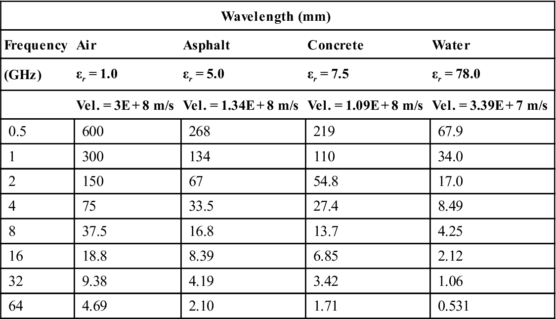
Table 8.1 lists wavelengths that are typically encountered in the use of GPR in various media. Technical advancements continue to ease testing at higher frequencies. The definition of high frequency is somewhat arbitrary, and continues to creep upward. One way of defining is to use an arbitrary cutoff frequency, such as 10 GHz. A similar, but perhaps more physically-based definition, is a specific wavelength value. Waves with lengths smaller than 10 mm have frequencies of 30 GHz and higher. It is common practice to use an inclusive factor of 10 in adjectival descriptions of wavelength and frequency. For example, millimeter waves have wavelengths of 10 mm or less, and terahertz waves have frequencies 0.1 THz (100 GHz) and higher.
Table 8.1
EM wavelengths as a function of frequency for different media
| Wavelength (mm) | ||||
| Frequency | Air | Asphalt | Concrete | Water |
| (GHz) | εr = 1.0 | εr = 5.0 | εr = 7.5 | εr = 78.0 |
| Vel. = 3E + 8 m/s | Vel. = 1.34E + 8 m/s | Vel. = 1.09E + 8 m/s | Vel. = 3.39E + 7 m/s | |
| 0.5 | 600 | 268 | 219 | 67.9 |
| 1 | 300 | 134 | 110 | 34.0 |
| 2 | 150 | 67 | 54.8 | 17.0 |
| 4 | 75 | 33.5 | 27.4 | 8.49 |
| 8 | 37.5 | 16.8 | 13.7 | 4.25 |
| 16 | 18.8 | 8.39 | 6.85 | 2.12 |
| 32 | 9.38 | 4.19 | 3.42 | 1.06 |
| 64 | 4.69 | 2.10 | 1.71 | 0.531 |
Most GPR systems use UWB EM pulses with very rapid rise and fall times to probe structures for subsurface features and damage. UWB technology dates back to the earliest days of radio communication with spark gap generators. The term ‘ultrawideband’ appears to have originated in an OSD/DARPA workshop in 1990 (MSSI, 2000). Most GPR UWB signals consist of a series of UWB pulses. This introduces two different frequency descriptors for the signals. The first is the frequency content of a single UWB pulse. Typical GPR UWB pulse widths run from 300 to 3000 ps. The corre-sponding frequency domain representation of narrow time domain UWB pulses is to cover a very broad frequency band (~ 0.5−10 GHz). The second frequency descriptor is the pulse repetition frequency (PRF), which typically runs from tens of kHz to 1 MHz or more.
In 1990, the OSD/DARPA Radar Review Panel issued a report establishing UWB radar as any system with a fractional bandwidth (FBW) greater than 0.25 regardless of the center frequency.
[8.1]
fH and fL are the upper and lower frequencies, respectively, of the –20 dB emission point (FCC, 2002). The average of the upper and lower frequencies defines the center frequency, fc, of the transmission.
[8.2]
Practical considerations led the Federal Communications Commission (FCC) to define UWB as signal with a FBW greater than 0.20 or a –10 dB bandwidth occupying more than 500 MHz of spectrum (FCC, 2002).
While there have been few, if any, credible reports of UWB GPR systems causing interference, the possibility of serious public safety consequences raises concerns. A NASA study demonstrated that UWB devices can interfere with commercial aviation navigation equipment (Ely, 2002). The tests found that a UWB transmitter with a 10 MHz PRF could interfere with aircraft navigation equipment using a carrier frequency approximately eleven times higher than the PRF. The exact mechanism of interference was not identified. One possibility is a high order harmonic of the PRF. This prompted the FCC to investigate and eventually to promulgate regulations for the unlicensed operation of UWB systems in the United States with the FCC 02–48 regulations (FCC, 2002; Olhoeft, 2002). The regulations established three general categories for UWB devices: imaging systems, vehicular radar systems, and communications and measurement systems. The imaging system category comprises GPR systems, wall imaging systems, through-wall imaging systems, surveillance systems, and medical systems. The regulations include the following guidelines:
• Applications – Imaging systems may not be used for data or voice information transfer.
• Operating Frequency – The operating frequency band is defined as the UWB bandwidth, i.e., the –10 dB emission bandwidth. GPRs and wall imaging systems must operate with this bandwidth contained below 10.6 GHz.
• System Operators – GPRs and wall imaging systems may only be used for law enforcement, firefighting, emergency rescue, scientific research, commercial mining, or construction purposes.
• Emission Limits – All imaging systems are required to comply with section 15.209 emission levels for frequency bands at or below 960 MHz. These emission levels are measured in terms of the field strength at a specified distance from the device. Table 8.2 lists the emission limits of 15.209 and provides a conversion of these levels to equivalent isotropically radiated power (EIRP) (NTIA, 2001). Table 8.3 shows the EIRP limits for radiation in bands above 960 MHz. Table 8.4 lists the limits for emissions measured using a resolution bandwidth of no less than 1 kHz.
Table 8.2
| Frequency (MHz) | Field strength (μV/m) | Measurement distance (m) | EIRP (dBm) |
| 0.009–0.490 | 2400/F (kHz) | 300 | 11.8-20 log10F (kHz) |
| 0.490–1.705 | 24 000/F (kHz) | 30 | 12.3–20 log10F (kHz) |
| 1.705–30.0 | 30 | 30 | –45.7 |
| 30–88 | 100 | 3 | –55.3 |
| 88–216 | 150 | 3 | –51.7 |
| 216–960 | 200 | 3 | –49.2 |
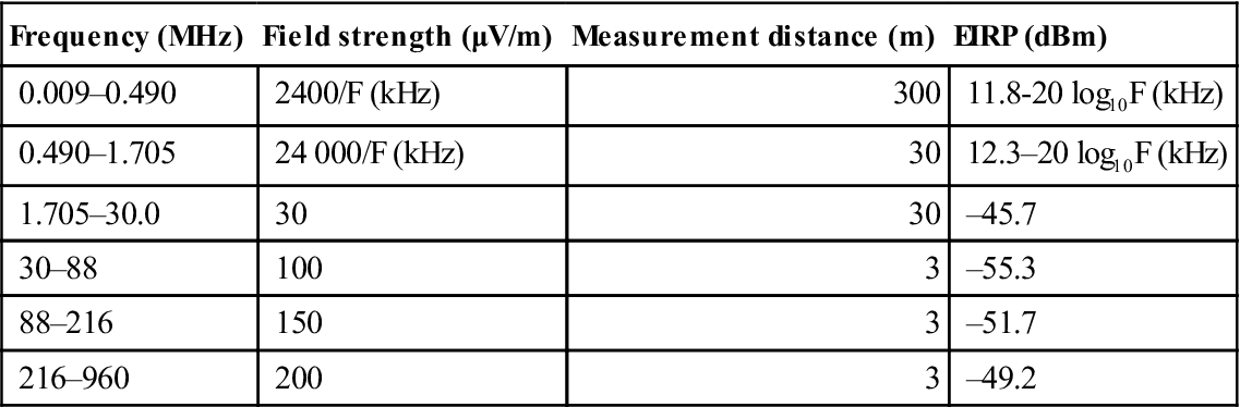
Table 8.3
Maximum average emission limits for frequency bands above 960 MHz
| GPR and wall imaging systems | |
| Frequency (MHz) | EIRP (dBm) |
| 960–1610 | –65.3 |
| 1610–1990 | –53.3 |
| 1990–3100 | –51.3 |
| 3100–10 600 | –41.3 |
| Above 10 600 | –51.3 |
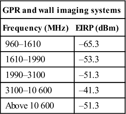
Table 8.4
Maximum average emission limits using a resolution bandwidth of no less than 1 kHz
| GPR and wall imaging systems | |
| Frequency (MHz) | EIRP (dBm) |
| 1164–1240 | –75.3 |
| 1559–1610 | –75.3 |

The limitations imposed by these regulations form a significant barrier to routine GPR operation, especially for applications that favor high PRFs and air-launched measurements, such as the sensing of subsurface roadway conditions at highway travel speeds. Nonetheless, technical workarounds are beginning to appear, e.g., full waveform digitization to reduce the PRF along with shaped UWB pulses (Xia et al., 2012).
8.3 Current challenges and state of the art systems
The state of the art is that a variety of commercial systems are available at a reasonable cost. The present systems continue to improve in terms of performance, ease of use, data processing, and presentation capability. Systems are available in a variety of frequency bands, some are over 3 GHz. Handheld units are increasingly usable and lower cost. For structural engineering applications, these systems are capable of inspecting roadways, tunnel walls, and building façades, locating buried utilities, and detecting water leaks in buried pipes.
There remain several technical challenges affecting the use of GPR for structural inspection. Automated data interpretation software has improved considerably, but much of the interpretation still requires considerable expertise. Vehicle mounted systems still use prohibitively large antennas. Penetration depth versus frequency and resolution tradeoff remains less than desirable. Source/receiver coupling is a persistent problem in impulse-type bistatic antenna systems. Measuring roadways at highway travel speeds with cm-scale spatial resolution while remaining compliant with emitted radiation level specifications, such as FCC 02–48, remains problematic. Cm-scale position registration without the prepositioning of supplemental navigational assist hardware is also a challenge.
8.4 Fundamentals of operation
EM wave propagation and interaction with materials underlies the operation of radar and millimeter wave systems, along with high-speed analog and digital signal processing. The mathematical modeling of EM fields can be highly technical. Different models with various degrees of rigor and complexity are available. Wisely choosing the physical model eases the analytical burden. Figure 8.4 shows a taxonomy of mathematical models, ranging from the relatively simple ray tracing models through scalar and vector waves to the fairly recondite quantum field models. At the moment, there are only a few situations related to GPR and millimeter wave sensing that require the power of quantum mechanics. An exception is the need for quantum techniques to design and model the solid state electronics that generate and receive EM waves (Taylor, 2001). The interactions of EM waves with materials are also quantum phenomena, but empirical models that fit within the framework of continuum-based Maxwell’s equations and simpler models seem to be adequate for most cases (Feynmann, 1977). An intriguing possibility is the use of Bell’s theorem in radar sensors (Allen and Karageorgis, 2008). The reader is referred to standard texts for more details on these topics (Moon and Spencer, 1960; Taflove and Hagness, 2005; Klauder and Sudarshan, 2006; Balanis, 2012).

Maxwell’s equations provide an excellent representation of EM phenomena on scales ranging from macroscopic to quantum. Maxwell’s equations treat the EM interactions in terms of electric and magnetic field vectors that propagate and reflect as waves. Often, scalars instead of vectors can represent the propagation of EM waves. Scalar forms simplify the mathematics at the expense of a loss of transverse directional information and cannot treat vector-based phenomena i.e. polarization. If the wavelengths are small compared to directional changes in propagation, then a geometric ray tracing model can be used. Ray tracing replaces the differential wave equations with geometric and trigonometric relations. A further simplification occurs if the media appear as a multi-layered planar structure with the wave direction being normal to the surface of the planes. This forms a 1-D multi-layered model.
Vector field equations describe many EM phenomena. The principal EM vector fields are the electric field, ![]() ; the magnetic field,
; the magnetic field, ![]() ; the electric displacement,
; the electric displacement, ![]() ; and the magnetic induction,
; and the magnetic induction, ![]() . In the absence of material discontinuities, these vector fields are normally finite, continuous, and differentiable functions of position and time. Heaviside’s version of Maxwell’s equations combines the four field vectors in a concise description of the field interactions
. In the absence of material discontinuities, these vector fields are normally finite, continuous, and differentiable functions of position and time. Heaviside’s version of Maxwell’s equations combines the four field vectors in a concise description of the field interactions
[8.3]
and
[8.4]
[8.5]
[8.6]
![]() is the source current density and
is the source current density and ![]() is the conductivity current density
is the conductivity current density ![]() .
.
In addition to Maxwell’s equations, EM wave descriptions also need constitutive material properties. In isotropic media, ![]() is parallel to
is parallel to ![]() , and
, and ![]() is parallel to
is parallel to ![]() , i.e.
, i.e.
[8.7]
and
[8.8]
ε and μ are the electrical permittivity and magnetic permeability, respectively. In a vacuum, or air at most wavelengths, ε0 = 8.854 × 10⁻¹² farad/m and μ0 = 4π × 10−7 N/A2, with the relation for the wave speed, c0, in a vacuum
[8.9]
Modeling the interaction of EM fields with anisotropic materials generally requires using tensor-based constitutive models.
For nonconducting and nondispersive homogeneous media, a condensation of Maxwell’s equations produces vector wave equations for both the electric and magnetic fields
[8.10]
[8.11]
c is the wave speed. The quantity (εμ0)1/2 is known as the refractive index.
These equations permit a wide variety of solutions, including plane waves of the form
[8.12]
φ and Φ0 are scalar components of the vector wave. ![]() is the wave number, which points in the direction of wave propagation.
is the wave number, which points in the direction of wave propagation. ![]() is the position in space. f = ω/2π is the frequency. Plane waves extend to infinity in the transverse directions. Feynman (1977) shows that for linear and homogeneous media, it is possible to represent almost any propagating EM wave via a superposition of different plane waves. Alternative formulations, such as spherical waves or Gaussian beams, are more tractable in particular situations (Verdeyen, 1989). Decomposing the propagating field disturbances with Fourier’s theorem and noting the linear nature of most wave propagation produces a simplified scalar sinusoidal waveform, d(x,t), that retains many of the essential features of wave propagation, where
is the position in space. f = ω/2π is the frequency. Plane waves extend to infinity in the transverse directions. Feynman (1977) shows that for linear and homogeneous media, it is possible to represent almost any propagating EM wave via a superposition of different plane waves. Alternative formulations, such as spherical waves or Gaussian beams, are more tractable in particular situations (Verdeyen, 1989). Decomposing the propagating field disturbances with Fourier’s theorem and noting the linear nature of most wave propagation produces a simplified scalar sinusoidal waveform, d(x,t), that retains many of the essential features of wave propagation, where
[8.13]
An examination of d(x,t) indicates that the instantaneous amplitude repeats when x/λ = ct/λ = 1. This leads to the definitions of λ as the wavelength (reciprocal of the wavenumber), and f = c/λ as the frequency.
EM waves propagate through a vacuum with no loss of energy or dispersion. The propagation of EM waves through all other media is lossy with a conversion of EM wave energy into other forms e.g. heat. A useful macroscopic representation of wave transmission losses is a linear model with complex-valued permittivities and permeabilities, i.e., ε* = ε׳ + jε" and μ* = μ + jμ" (Condon and Odishaw, 1967).
[8.14]
The propagation factor, γ, is
[8.15]
α is the attenuation factor (α = 0 for loss-free media). β is the phase factor, which indicates the phase velocity of the wave. For most dielectric materials, it is reasonable to absorb the loss factor into the imaginary part of the permittivity ε*, which leaves a real expression for the magnetic permeability. A useful and relatively easy to measure version of the loss factor is the loss tangent, δ = ε″/ε′. Using complex-valued loss functions is generally appropriate only in the context of oscillations with stationary frequency content, e.g. harmonic inputs and outputs. Using complex loss function models in transient analyses can cause anomalous non-causal behaviors. Purely imaginary dielectric values correspond to strong reflections and are useful for modeling metallic surfaces.
An antenna produces EM field disturbances by driving time-varying electric currents through conductive elements. The motion of the electric charges induces time-varying magnetic fields, which in turn induce time-varying electric fields. The repeated interchange of space-and time-varying electric and magnetic fields propagates the EM field. The near-field region is the space near the antenna where the initial magnetic fields form. The size of the near-field is typically in the order of one wavelength. The reactive near-field is a quarter wavelength or less. The far-field is typically two wavelengths or more away from the antenna. A transition region lies in between. The distinctions between near-field and far-field are not crisp and depend on the geometry and other details of the antenna design. The concept of reactive near-field is particularly important in ground-coupled antennas.
For GPR applications, ray tracing methods can provide insight into the interactions of EM waves with layered media and bulk conductors, especially when the transverse spatial variation of dielectric properties occurs over lengths that are larger than several wavelengths. These methods use rays (directed lines) to describe the propagation of EM field disturbances. An important application is to use rays to describe the hyperbolic nonlinearity that is characteristic of an isolated reflector in a B-scan. A GPR identifies the presence of a reflector by measuring the time, Δt, for a wave to launch, reflect, and return. Denoting r as the distance from the antenna to the reflector gives
[8.16]
cm = the speed of light in the medium. The factor of ![]() appears in Equation [8.16] because the wave has to make a round trip. Equation [8.16] is particularly useful if the reflector is known to be directly down range of the antenna, or if the reflector is planar, such as a layer of material with a refractive index that is different from the one above it. If the reflector is isolated and is positioned laterally from the source antenna, then Equation [8.16] is still valid, but the travel distance, r, is the diagonal distance from the antenna to the reflector (Fig. 8.5).
appears in Equation [8.16] because the wave has to make a round trip. Equation [8.16] is particularly useful if the reflector is known to be directly down range of the antenna, or if the reflector is planar, such as a layer of material with a refractive index that is different from the one above it. If the reflector is isolated and is positioned laterally from the source antenna, then Equation [8.16] is still valid, but the travel distance, r, is the diagonal distance from the antenna to the reflector (Fig. 8.5).
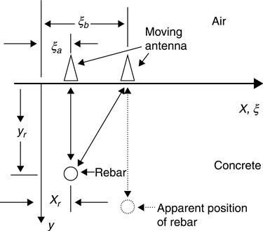
From a single trace, it is not possible to discern simultaneously the cross-range and down-range position of an isolated reflector. If it is erroneously assumed that a reflector is immediately down range from the antenna, when its position actually has a cross-range component as well, then the apparent position of the object is directly down range at a distance equal to combined down-range and cross-range position. The time for a signal to travel round trip from the antenna to the reflector is
[8.18]
Moving the antenna across the surface, collecting a series of scans, stacking the scans, and plotting the amplitude in terms of pixel brightness produces a B-scan.
For a fixed-position reflector, Equation [8.18] forms a hyperbola in ξ and Δt. Figure 8.6 shows the hyperbolae that result from having a reflector at various depths. Deeper reflectors produce a hyperbola with flatter appearance.
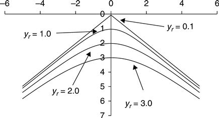
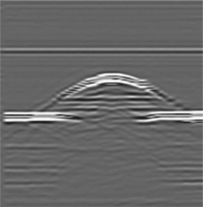
Figure 8.7 shows a B-scan image of the reflections from a round aluminum bar suspended in air.
A polarized EM wave with the electric field vector parallel to the x-y plane and the magnetic field parallel to the x-z plane is a transverse electric (TE) polarized wave. When the wave is polarized so the that the magnetic field vector is parallel to the x-y plane and the electric field vector lies in the x-z plane, the wave is called a transverse magnetic (TM) polarized wave. TE waves and TM waves interact differently with a boundary between materials with differing refractive indices, n1 and n2 (Udd, 1991). The reflection (R) and transmission (T) coefficients are
[8.19]
[8.20]
[8.21]
[8.22]
When the angle of incidence θI = 0, the situation corresponds to testing in a monostatic (single antenna) mode with layered media. Equations [8.19] to [8.22] simplify to
[8.23]
[8.24]
If the two media are dielectric and if it can be assumed that the change in wave speed is due to changes in the dielectric permittivity constants (rather than the magnetic permeabilities), the reflection and transmission coefficients for a wave traveling from medium 1 to 2 are
[8.25]
[8.26]
If ε1 is less than ε2, then R12 has a negative value. If ε1 is larger than ε2, then R12 is positive. The magnitude of the reflection coefficient dictates the amplitude of the reflected wave, and the sign of the reflection coefficient dictates the phase shift of the returning wave. When R12 is negative the incident wave undergoes a 180° phase shift upon reflection. When R12 is positive, no shift in phase occurs (Carter et al., 1986). Setting the dielectric constant ε2 to infinity models the reflection from a metal surface. In this case R12 = –1 and T12 = 0.
The different reflectivities of a dielectric surface and a metallic surface provide a means to determine the dielectric constant of a roadway surface. Denoting A as the amplitude of the reflection from a normal incidence wave off of the surface of the roadway and APL as the amplitude of the reflection off of a metal plate placed on the roadway surface gives the dielectric constant for the roadway as
[8.27]
Many cases of EM modeling are intractable with analytic tools. Numerical methods often provide a viable alternative. The finite difference time domain (FDTD) method models transient EM waves (Yee, 1966; Taflove and Hagness, 2005). A drawback is that stable and convergent solutions often require small grid spacings and high computational loads. Many practical situations restrict FDTD solutions to 2-D.
8.5 Electromagnetic interactions with materials
Many of the interactions of EM waves with homogeneous materials depend on a combination of the atomic nature of the material along with the frequency of the waves. The mobility of the electrons at the atomic scale governs many of the constitutive properties. If the electrons are free to move, as in a metallic conductor, they will move to counter the action of EM waves. The effect is that metals reflect EM waves and do not permit much penetration of the EM fields past a skin on the surface. Alternative atomic arrangements bind most of the electrons into molecular structures. In these cases, EM waves cause the molecules to rotate and align internal charge gradients with the external fields. This effect gives rise to dielectric materials (Debye, 1960). If the molecules rotate elastically, then the input energy regenerates and the material is a lossless dielectric. If the rotations convert energy into heat, the material is a lossy dielectric. GPR models commonly use four types of EM properties:
1. Vacuum or air: The EM properties of air and a vacuum are virtually identical for the frequencies and transmission distances commonly encountered in GPR. EM waves propagate through air with minimal losses.
2. Dielectric: Dielectrics are insulating materials containing dipoles. Electric fields exert moments on dipoles, often in proportion to the strength of the field,
[8.28]
![]() is the electric displacement vector, εr is the dielectric constant for the material, and
is the electric displacement vector, εr is the dielectric constant for the material, and ![]() is the applied electric field. The permittivity of air is often normalized to unity and the dielectric constant εr is also normalized, with a value that is always greater than or equal to one.
is the applied electric field. The permittivity of air is often normalized to unity and the dielectric constant εr is also normalized, with a value that is always greater than or equal to one.
3. Lossy dielectric: Ideal dielectrics allow the propagation of EM waves without any losses. All real passive materials produce losses, which convert the EM energy into heat and attenuate the amplitude. A linear model with complex-valued permittivities and permeabilities is the usual approach to modeling the loss mechanisms.
4. Metallic reflective: Free electrons in metals move quickly to counter incoming EM waves. This gives metals a shiny appearance and makes them reflect light and other EM waves. It is common to use a dielectric constant of ∞ for metals.
The deterioration of concrete and asphalt often changes the EM constitutive properties. Many damage features are smaller than 1 cm, which is smaller than the spatial resolution of most GPR systems. This limitation in resolution reduces the ability of radar to detect the fine dielectric discontinuities that result from deterioration mechanisms and instead leads to bulk continuum models of dielectric properties. Halabe et al. (1990) developed a model to characterize the complex dielectric constant of asphalt and concrete mixtures as a function of wave frequency, sample temperature, moisture content, chloride content, and mix constituents. The model calculates the dielectric permittivity of concrete from the known permittivity of its discrete constituents (i.e., aggregate, air, water, chloride, cement paste). Although water and salt compose a relatively small percentage of a given concrete or asphalt pavement sample, the effect on the permittivity can be quite large. Unbound water molecules increase the average dielectric constant of the material. Salt and other ionic substances increase the attenuation of traveling EM waves (Al-Qadi et al., 1995). Several models predict the dielectric properties of a mixture from the properties and volumetric proportions of the constituents (Halabe et al., 1993, 1995). The components in these models include coarse and fine aggregate, cement paste, air, water, and salt. Water and salt, only when dissolved in solution, have the greatest effect on the dielectric constant. A form of the Debye expression for the relative dielectric permittivity of salt water (εsw) is
[8.29]
εo = static dielectric constant of the solvent, ε∞ = high-frequency dielectric constant of solvent, τ = relaxation constant, σ = conductivity of water, and f = EM wave frequency. Water plays such a large role because the dielectric constant (≈ 80) is much greater than that of dry natural rock, soil, and concrete (2.5–8.0).
The complex reactive index mixture (CRIM) method assumes a volume average of the complex refractive indexes of the constituents.
[8.30]
ϕ = porosity of concrete = (volume of voids)/(total volume of concrete), S = degree of saturation = (volume of water)/(volume of voids), εm = relative dielectric permittivity of concrete solids ~ 5.0 (real), εa = relative dielectric permittivity of air = 1.0 (real), εsw = relative complex permittivity of water, and εr = relative dielectric permittivity of resulting concrete mixture = εI + iεII.
8.6 Transmitter and receiver design
GPR systems generally fall into two main classes for the transmitter and receiver design. One is based on using short EM impulses. These are known as impulse radar systems. The second class uses sinusoidal waves that sweep over a range of frequencies, and are known as step-frequency or continuous-wave radar systems. Most commercial GPR systems are impulse radars. Many academic researchers favor step-frequency systems. Other transmit/receive designs are in use, such as noise-modulated radar (Reeves, 2010).
The advantages of impulse systems lie mainly in the ability of a single impulse wave to produce a return wave that is laden with information describing subsurface features. Impulse systems are fast. The high speed is a mixed blessing. It enables rapid testing, but requires high-speed electronics for measurement. Traditional methods use sub-sampling to take a single data point sample from an impulse waveform and reconstruct a complete waveform from average samples from multiple waveforms. Full waveform single-shot digitization has been demonstrated using high-speed analog to digital conversion (ADC). In order to achieve reasonable sampling speeds, most full waveform digitizing instruments use sample and hold amplifiers to multiplex the signals to a gang of slower ADCs to form a single-shot reconstruction. Figure 8.8 shows the full waveform digitization of a 1 ns impulse using a gang of ADCs with a sampling rate of 20 GHz.

The advantages of step-frequency systems are the ease of increased dynamic range and good control of the frequency content of the outgoing waves. Disadvantages include a slower signal acquisition speed, the need to convert the frequency domain data to the time domain with digital Fourier transforms, and that the instruments tend to be more expensive.
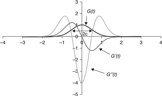
A good approximation to the shape of impulse is the Gauss bell, G(t),
[8.31]
The coefficient A determines the height of the impulse. A measure of the width is 2c. Derivatives of the Gauss function are known as Gauss-Hermite functions, Fig. 8.9 (Wiener, 1958). The first derivative, G′(t), is known as a monocycle or doublet. The second derivative G″(t) is known as a Mexican hat function (upside down in Fig. 8.9).
A useful property of the Gauss function G(t) is that the Fourier transform is also a Gauss function, i.e. (Papoulis, 1968):
[8.32]
This relation confirms that impulses have broadband frequency content. Narrower width impulses produce broader width frequency content. A 1 ns pulse has the bulk of its spectral energy in a region less than 1 GHz.
Creating impulses requires high-speed electronics. There are two primary methods. SRDs form the basis of one set of methods. SRDs are key components in MIR systems (McEwan, 1994b). Avalanche transistors form the basis of the second set (Morey, 1974). SRDs tend to produce low power outputs, and consume small amounts of power. Avalanche transistors can produce larger amplitude pulses, but consume more power.
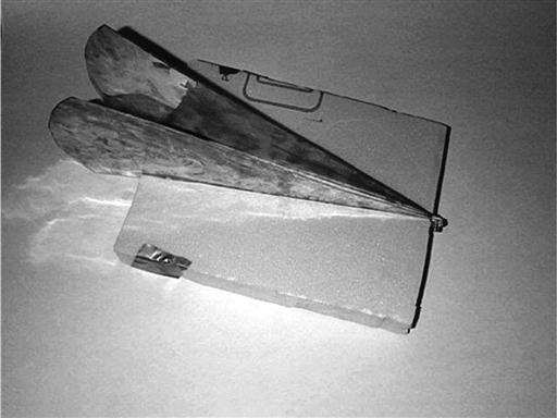
Antennas launch and receive the EM waves. Collecting high quality signals depends on the ability of the antennas to direct and control the waves with minimal distortion and signal loss. Most GPR antennas operate in air-launched, ground-coupled and borehole configurations. Air-launched antennas pass EM waves through the air on both the send and receive paths, with about 50% of the signal strength being lost due to surface reflections (Smith, 1995). Most air-launched antennas have a horn geometry, Fig. 8.10. Air-launched antennas often stand 0.3–1.0 m above the ground for pavement studies. A notable exception is airborne GPR instruments, with much larger standoffs. The stand-off air-launched geometry is convenient in applications that require moving the antennas across the ground surface. Ground-coupled antennas operate in close enough proximity to couple reactive near-field EM interactions directly into the ground. The typical geometry is a ground-flush mount at a gap of a few cm at most. Reactive near-field coupling enhances signal transmission and reception strength. Borehole antennas place the antenna in a hole drilled into the ground and also use near-field coupling of the EM waves. Most of the ground-coupled antennas have a bowtie geometry, which is essentially a some-what smaller and flattened horn. Figure 8.11 shows a GPR-based roadway inspection system that uses specialized ground-coupled antennas that can move at driving speeds. The mechanical design enables this system to combine the increased signal transmissibility of ground-coupled antennas with the mobility of an air-launched antenna to realize a 46-wide antenna array capable of producing a 3D array image, with a data density of 50 mm across the road, and 50 mm along the road, down to a depth of 1.2 m, all at 100 km/h.

Impedance matching is one of the more important concerns in the design and fabrication of radar antennas. Impedance matching has a large effect on performance, often with significant frequency-dependent effects. Impedance mismatches along a signal path causes reflections. Reflections due to impedance mismatches can contain valuable information concerning the type and geometry of subsurface features in a solid under test. When the impedance mismatches occur in the cabling and the antenna, the reflections do not contain useful information and are a source of power loss, which reduces the penetrating depth and effective resolution of the system. The voltage standard wave ratio (VSWR) quantifies the mismatch in terms of the ratio of the amplitude of the reflected voltage wave to the amplitude of the incident voltage wave, Γ.
[8.33]
When the value of the VSWR closely approaches 1, the impedance match is satisfactory. If the impedance is totally mismatched, Γ is 1, and VSWR approaches infinity. Nominally acceptable values of the VSWR run between 1 and 2.
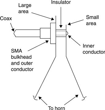
In an antenna, the impedance match at the apex and the impedance match at the aperture are of primary concern. The apex connects the antenna to the feed cables and then to the analyzer. A design goal for the apex is to minimize the reflections that occur with the impedance mismatch as the coaxial cable is connected into the antenna. The geometry of the coaxial cable, and the unipolar nature of the source signals, makes it difficult to create an impedance-balanced connection by directly attaching the source to the antenna. One option is to use a balun to convert from a unipolar to a bipolar format. However, total losses with baluns are typically 20 dB for a round trip signal. An alternative is to balance the connection by the inclusion of specific geometric details in a direct connection. Balanis (1997) lists several such balun direct-connect configurations. With care, an apex geometry can be found that produces a negligible impedance mismatch, such as that of Fig. 8.12. Blended geometric forms and resistive loading are standard methods of reducing impedance mismatch at the aperture (Huston et al., 2000b).
8.7 Signal processing
A typical single GPR measurement collects a trace of an EM signal that reflects back from the solid under examination, Figs 8.1 and 8.2. Repeating the measurement with the antenna placed at a different point produces a measure of the reflectivity of subsurface features from a different point of perspective. The change in geometry can provide new and useful information. Taking measurements at a series of points by moving a single antenna or with a multi-antenna system gathers even more information. Condensing the data into useful information-dense formats is a primary task of GPR signal processing. The most common of these is a B-scan that presents a series of traces taken from a set of points along a line.
The 2-D and 3-D nature of radar signals and subsurface features often makes it difficult to discern the nature of the underlying features from a direct examination of the B-scan images. A major difficulty is the distortion due to hyperbolic nonlinearities that result from the extended distance of cross-range objects (Fig. 8.6).
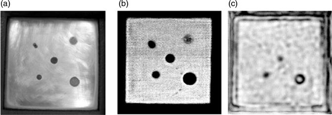
The development of 2-D and 3-D imaging algorithms with applicability to GPR occurred along two independent paths – geophysical oil exploration and airborne radar. The geophysical oil exploration algorithms usually go by the name ‘migration’ (Stolt, 1978; Robinson, 1982). The airborne radar applications are usually called ‘SAR.’ Migration and SAR refer to a whole set of algorithms that attempt to deconvolve hyperbolic nonlinearities by various integral transforms and manipulations of entire sets of B-scan data. One of the earlier reported applications of the SAR technique to the imaging of subsurface features in concrete is by Mast (1993). Mast and Johansson (1994) further extended this work into 3-D imaging of subsurface features. Johansson and Mast (1994b) describe a related approach using multi-frequency diffraction tomography. Figure 8.13 shows the results from a test on a slab with embedded steel reinforcing bars and dielectric targets. The system is able to image the reinforcing bars and dielectric targets quite nicely. Imaging defects, such as cracks and corrosion, is more difficult.

A flowchart for the basic SAR algorithms as described by Soumekh appears in Fig. 8.14. A key feature is that combined Fourier transforms in the frequency and wave number domains algebraically remove the hyperbolic nonlinearity B-scan data (Soumekh, 1999).
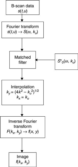
The geometry of the hyperbolic nonlinearity in wave number space is shown in Fig. 8.15. The key relations are
[8.34]
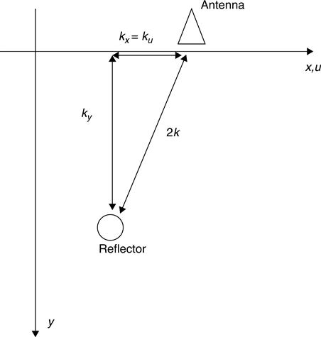
or
[8.35]
and
[8.36]
where kx = down-range image wavenumber, ky = cross-range image wave number, ku = down-range wave number, and k = ω/c = wave number. This transforms the data into a form that represents the geometry of the reflective features. Finally, the data are inverse Fourier transformed into the spatial x-y domain to form an image.
8.8 Laboratory and field studies
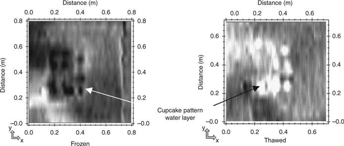
Water intrusion is believed to be a major factor in many progressive damage modes in roadways and structures. One method of detecting subsurface water is to note that the transmissibility at 2.4 GHz changes with phase. Liquid water absorbs EM waves at 2.4 GHz. This is the basis for microwave ovens. Frozen water is transparent at 2.4 GHz. Figure 8.16 shows the results of a test on concrete slabs with water-filled variable and uneven depth layers. Water in the form of saturated towels was placed on top of the cupcake plateaus and in some of the flat surfaces between the slabs. The relative absorption of the thawed versus frozen patterns is distinctive.
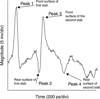
The ability of GPR to reliably detect delaminations between layers in concrete and asphalt structures remains to be established with certainty. Figure 8.17 shows the results of a laboratory study that boosts the possibility. The test used slabs of concrete with 1 mm gaps to simulate a delamination. A 1–16 GHz impulse GPR system was able to detect the 1 mm air-filled gap. It should be noted that delaminations encountered in the field often have rough surfaces, and not the smooth surfaces encountered in this test. The cupcake patterns of Fig. 8.16 were part of a test regime that looked into some of these questions.
In an effort to clarify further the ability to detect corrosion damage with GPR and other sensors, a series of studies were conducted at the Federal Highway Administration (FHWA) NDE Laboratory (McLean, VA, USA) (Cui, 2012). These tests involved inducing accelerated corrosion in a reinforced concrete slab with weekly ponding, removal, and drying of saline water over the course of a year (Fig. 8.18)
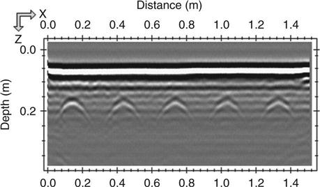
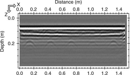
A B-scan of the slab after six months of curing and before the accelerated corrosion test appears in Fig. 8.19. Hyperbolas corresponding to subsurface reinforcing bars are distinct. A B-scan of the slab after seven months of accelerated corrosion testing appears in Fig. 8.20. The hyperbolas corresponding to subsurface reinforcing bars are somewhat fuzzy. This confirms the hypothesis underlying AASHTO TP36–93 that corrosion damage causes a blurring of the reinforcing bar hyperbolas (AASHTO, 1993). However, the mechanisms that produce this blurring remain undetermined. Subsequent dissection of the slab indicated that there was minimal cracking, no delaminations, and that the amount of corrosion surrounding the reinforcing bars was approximately at Stage 4 in Fig. 8.3. Rapid chloride testing of the concrete post mortem found concentration levels of chlorides in excess of 0.5% by weight. Overall, the results of these tests indicate that GPR can likely be useful in detecting early stage concrete chloride-induced corrosion damage.
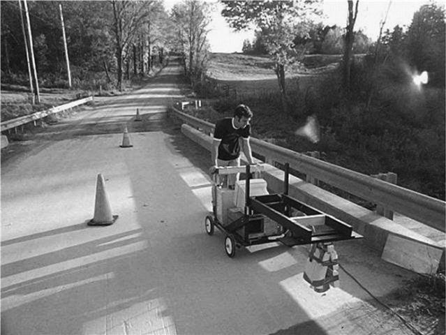
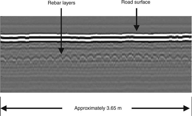
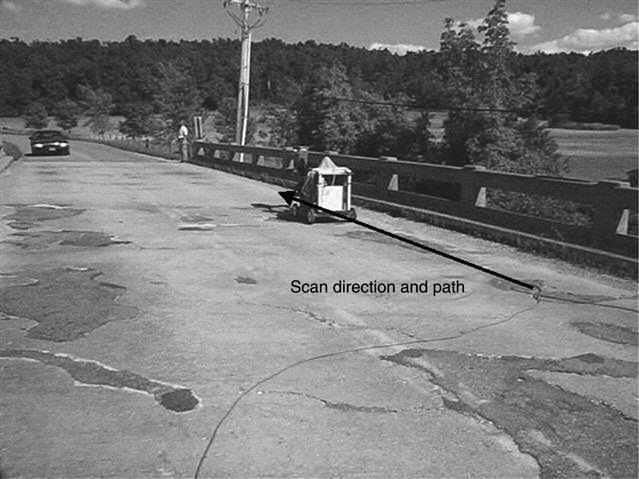
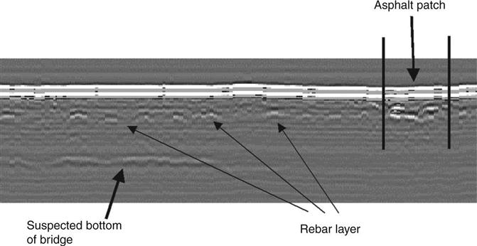
A field test of a newly constructed healthy bridge deck appears in Fig. 8.21, along with a B-scan showing distinct hyperbolas from reinforcing bars in Fig. 8.22. These figures contrast with those of the Bostwick Road Bridge, Shelburne, VT, USA, Fig. 8.23. The reinforcing bar hyperbolas are barely discernible in this distressed bridge (Fig. 8.24).
The high-frequency range of EM wave NDE technology presently extends into the terahertz range. Many materials quickly attenuate terahertz EM waves, which limits their utility for subsurface probing. However, there are some applications where terahertz sensing is useful. These generally involve detecting features underneath a relatively thin outer layer that is transparent to terahertz waves. Detecting corrosion under thermal protection system (TPS) tiles or paint is a good candidate for terahertz sensing tests. Figure 8.25 shows the ability of a 75–100 GHz system to detect corrosion under a 25.4 mm thick Space Shuttle TPS tile.
8.9 Conclusions and future trends
The ability to launch, control, and measure EM waves with increased levels of sophistication at relatively low cost opens up new opportunities and sensing modalities. Of particular note is the use of interferometric radar to monitor remotely the dynamic motions of large structures, such as bridges (Mayer et al., 2010). A vibrant trend is the appearance of multichannel systems, which offer the opportunity for increased data collection rates. For example, a multichannel system can inspect a full road lane in a single pass, rather than multiple passes, as required with a single or dual-channel system. Coarse-pitch antenna arrangements essentially have the antennas operate as a set of independent single antennas. Dense-pitch arrangements, with the between-antenna spacing at less than one quarter wavelength, allow for tomographic reconstructions that avoid excessive interpolations (Grasmueck et al., 2005). Another trend of note is the concept of periodic nondestructive testing (NDT), which subjects structures to repeated examinations to ascertain long-term trends and significant changes in the condition (Jalinoos, 2009). Affordable and easy-to-use instruments are an essential ingredient in periodic NDT. The increased use of digital signal processing techniques, such as high-speed ADC, may facilitate more periodic NDT approaches (Xu et al., 2013).
An interesting possible future development will be the adaptation of cognitive radar system concepts to GPR systems (Haykin, 2006, 2012). A cognitive GPR system uses information gathered from real-time data analysis to provide information to the system controller for resetting the operational parameters to ensure optimal data collection performance. The technique uses the four primary actions of perception-action, memory, attention, and intelligence. A simple example would be a roadway inspection GPR that changes operating parameters based on a perception as to whether it is traveling on a road or on a bridge deck. Roadways may be best examined with low frequency waves at a fairly coarse pitch to penetrate and measure subbase conditions. Bridge decks may be best examined with a finer level of attention using high-frequency fine pitch measurements. Similarly the gains on the receiver hardware may be optimally selected by the cognitive system. A more sophisticated controller may be one that selects operational parameters based on what gives the best level of resolution and information content. The mode selection may be driven by a combination of navigational and data driven estimates of state. At the heart of the controller is an operational parameter-setting matrix that serves as a map from a discrete set of environmental (observational) condition states onto a discrete set of operational parameter states. Upon perceiving an environmental state, the controller uses the map to select the operational parameters. The process iterates as the system encounters new environmental state. A simple approach is to use an intelligent designer to preselect a static map. A more sophisticated, but possibly better, approach uses machine learning to update the map dynamically. Updating methods include greedy and reinforcement techniques that alter the map in a positive response to parameters that improve performance (Bongard et al., 2006; Christensen et al., 2010) and the motivational methods that attempt to reduce negative responses in a method analogous to pain avoidance (Starzyk et al., 2012).
It has been proposed that corrosion of steel inside concrete produces nonlinear effects that can be measured by sub- and super-harmonic methods (Kwun, 1993). To date, however, nonlinear interactions of materials with EM waves have not been extensively studied. A primary reason is the lack of suitable test instruments and protocols. The recent appearance of non-linear vector network analyzers and the development of algorithms based on polyharmonic distortion coefficients (X-parameters) in the frequency domain and Volterra series in the time domain may prompt future developments in this area (Verspecht and Root, 2006).
Additional areas of active and possibly fruitful research include developing multisensory data fusion methods that combine the strengths of GPR sensing with those of other sensors to produce better renditions of structural conditions (Huston et al., 2011), and the development of less bulky electrically small antennas.
In conclusion, radar technologies are sufficiently mature to be able to provide useful information to users of the instruments, and technical improvements and innovations are proceeding on active paths that should lead to improved performance along with a wider range of usage.