Objects in statics can be subjected to a wide variety of actions from an almost infinite list of sources. Having the ability to transform a system of many similar effects into a single equivalent behavior (called a resultant) is a truly handy skill.
Resultants aren't necessarily a cause-and-effect relationship. If you sit on a tiny, cushy kiddie chair (cause), the outcome (result) would likely be that the chair may be a bit lumpier (or in a few more pieces) than it was before.
In statics, the resultant behavior has a different meaning. Resultants represent a way of consolidating information. For example, if you sit on the kiddie chair and your friend comes in and sits on the chair at the same time, the statics resultant is that two people are applied at the same location (on your chair), or that twice the number of loads have been applied to your chair.
In this chapter, I show you several different methods for determining a statics resultant, each of which requires different techniques. Some of these methods can be labor intensive yet light on mathematical requirements, and others are more complex yet robust. However, being able to consolidate multiple vectors into one combined vector makes your calculations so much easier. Picture a statics problem as a cage full of hyper kittens — if you open the cage, the kittens run out in any number of directions and at different speeds. That's a lot of different vectors at work! Resultants give you the ability to substitute those hyperactive critters with a single replacement. In simple terms, why deal with a hundred different actions when you can deal with just one?
A resultant vector (or simply a resultant) is the most basic representation of a system of combined actions that result in the same behavior as the original system. Often, this equality means you combine multiple vectors into a single equivalent vector.
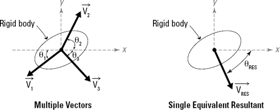
The first part of Figure 7-1 shows an object subjected to three separate actions in three different directions. With all of those actions combined, the body should experience a single response in a unique direction. That combined response is illustrated in the second part of the figure by VRES and is oriented at its own unique angle θRES.
Note
The resultant vector's magnitude (numerical value) and orientation (combined sense and direction) are uniquely determined by the magnitudes and orientations of the original uncombined vectors.
The position vector I discuss in Chapter 6 is actually a type of resultant vector. It starts at a given location and ends at a second point. However, a position vector actually has an infinite number of paths (if you ignore walls, fences, and other physical barriers) to get from one point to another. The position vector is the simplest representation of a path from one point to another, independent of which of the individual pieces you use.
The resultant calculations for a vector are the same regardless of the type of vector. Force vectors, velocity vectors, and displacement vectors can all be combined with similar types of vectors to create resultants. But before you start combining force vectors with displacement vectors to calculate resultants, keep a couple of simple guidelines in mind:
Only vectors of similar types may be combined to create resultants. A resultant vector is the same vector type as the vectors that create it. Force vectors can only be combined with other force vectors — you can't combine a force vector and a velocity vector to produce a position vector resultant.
Magnitudes and directions of resultant vectors can be larger, smaller, or the same as any of the combined vectors. The magnitude and direction (sense) of a resultant vector are directly related to the properties of the vectors that are combining to make the resultant. Two large vectors in opposite directions may produce a very minimal resultant effect.
Note
Because a resultant is also a vector and has been created from combining smaller vectors, it has its own magnitude, sense, and point of application, which are a direct result of the vectors that helped create the resultant. For more on these properties, look at Chapter 4.
You can calculate the magnitude and direction of resultant vectors in many valid ways. Generally, these techniques fall into one of three categories: graphical methods, geometric methods, and vector equation methods.
Graphical methods: Graphical methods typically include making a detailed sketch (drawn to scale) of all the vectors in the system you want to determine the resultant for. You then make a physical measurement from the drawing to determine the solution.
Geometric methods: Geometric methods use basic sketches and geometric principles to determine the resultant of two vectors.
Vector equation methods: Vector equation methods use Cartesian vector notation (from Chapter 4) to determine the resultant of a system of vectors. They require the vector mathematics I explain in Chapter 6.
The most common way to illustrate a system of vector actions is the head-to-tail construction I first discuss in Chapter 6. This construction technique is very useful in each of the three major resultant construction techniques that I describe in the coming sections. You can perform the head-to-tail construction method by using the following steps:
Select an arbitrary starting point.
The origin of your coordinate system is often a convenient starting point, but you're not required to use that point. However, you must choose an origin somewhere.
Choose any one of the original vectors and place its tail at the starting location you determined in Step 1, making sure to maintain the original orientation and sense.
You can start with either vector, but after you use a vector one time, you can't use it again. You must keep the same magnitude and direction for each vector.
Select one of the remaining original vectors and affix the tail of that vector to the head of the vector from Step 2.
Keep attaching vectors to each other (by repeating Steps 2 and 3) until you've used all of the original vectors.
Tip
The order of selection for the vectors that you choose in Steps 2 and 3 isn't important. You can use them in any order, but you can only use a vector once in this technique, and you must use all vectors.
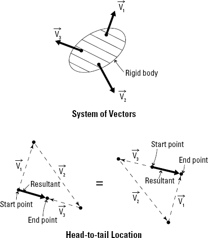
Consider the system of vectors in Figure 7-2, which shows a rigid body with three vectors acting on it. There are multiple ways to find the resultant using the head-to-tail method. For illustrative purposes, I show you two different possibilities for constructing the resultant of the system of vectors. Notice that the final vector has the same magnitude, sense, and line of action for all cases.
The easiest method for determining the resultant of a system of forces is to create a scaled drawing. Graphical methods are very convenient because they typically require you to perform very few mathematical calculations and you don't need a vector formulation at all. If you can draw a line at a specified length and angle/direction, you can determine the resultant. Plus, this method can handle multiple vectors at once. Computer aided drafting (CAD) programs and hand drawings with rulers, protractors, and compasses provide useful tools for these techniques.
The graphical methods do have their drawbacks, though. They're time- consuming to draw, and you can really only use them on two-dimensional problems. Although you can theoretically use this method in three dimensions as well, it's definitely not an easy (or efficient) method for those problems. Graphical methods also require a computer or mechanical drafting tools, and you can't guarantee their numerical accuracy because your tools are only so accurate (mechanical protractors are accurate to about one-degree increments, and your magnitude measurements are always limited by the scale of your ruler). As CAD systems have become more popular, you can actually use CAD drawings to achieve more accurate numerical measurements of the magnitude and direction of the resultant. Despite some of these accuracy issues, graphical methods can provide an effective (and often quick) qualitative view of size of the magnitude and general direction of a resultant vector.
The actual procedure for construction of a graphic representation of a resultant vector is fairly straightforward. Consider the rigid body of Figure 7-3a. In this example, notice that the magnitude of each force vector is given and that the directions of those vectors are described by either angles or proportions.
To perform this construction, you utilize the head-to-tail construction technique from the preceding section with a couple of minor modifications. Just follow these steps:
Choose your starting point and establish a grid for construction; indicate that your scale is one grid square represents one vector unit.
Select one of the two vectors and affix its tail to the starting location of Step 1.
In Figure 7-3b, I've arbitrarily chosen to start with the 1.41-Newton force. Be sure to precisely draw the force at its true scale length of 1.41 Newton at an angle of 45 degrees from the start point.
Warning
Preserving the proper magnitude and direction angles in your sketches is very important. If your sketches aren't accurate, you can't expect your final measurements to be accurate!
Sketch the next vector to scale at the proper orientation; repeat for any additional vectors.
Start by laying in the line of action (line in space where the vector is acting) of the force. You can easily find this line in the example in Figure 7-3b because you actually know the proportions of the grid.
To establish this line that passes through the end point of the vector from Step 2, follow these steps:
Locate a second point by counting down the number of grid squares on the vertical leg of the proportion triangle (which I discuss in Chapter 5) and then counting over the number of grid squares that are on the horizontal leg of the proportion triangle.
Draw a continuous line of action through these two defined points to establish the direction of the vector you're working with and then measure a distance that has the same length as the magnitude of this vector along the line of action from the end point of the vector in Step 2.
In the example, you measure five units from the end point of the"1.41-Newton force. This new point is the head location for the"5-Newton force.
Draw your vector arrow from the tail point to the new head location.
Sketch the resultant by drawing a vector arrow from the start point of Step 1 to the end point of the last vector that you drew.
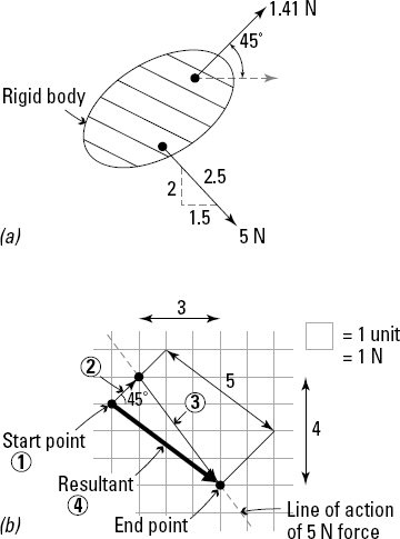
Congratulations — you've determined the direction of the resultant vector! You can now use a protractor to measure the angle of the resultant vector relative to a horizontal gridline, a vertical gridline, or even one of the original vectors' lines of action. The choice is yours. To determine the magnitude of the resultant, you simply need to use a ruler to measure the length of the resultant vector's arrow on your grid.
To avoid the problems inherent in graphical solutions (see the preceding section), geometric methods can present a better estimate of the magnitude and direction of a resultant. They don't require vector formulations, and the solution method is very, well, methodical. Unfortunately, these techniques only work effectively on two-dimensional problems and only on a maximum of two vectors at a time (although you can repeat the process with your resultant and additional vectors until only one resultant remains).
The most popular geometric construction technique is dubbed the parallelogram method because it incorporates an actual parallelogram into the solution process. However, you need to master several trigonometric identities to use this technique, so I tackle those in the following sections before showing you how to create the resultant.
By far the most essential geometric identities you need, aside from SOHCAHTOA (which I explain in Chapter 2), are the law of cosines and the law of sines. Each of these methods utilizes angle and dimensional relationships for triangles such as the one shown in Figure 7-4, which shows a triangle 123, having sides of length A, B, and C and corresponding opposite angles of a, b, and c, respectively.
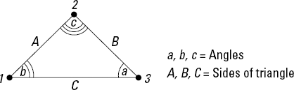
The law of cosines provides a formula that relates two sides and an included angle (an angle between two adjacent sides of a polygon) to the length of the third side. These formulas can be expressed as
Notice in Figure 7-4 that each of these expressions includes the length of two sides, and the angle between those same two sides. From this information you can then determine the length of the third side.
Tip
You must know at least two sides and the angle between those two sides to compute the third side by using the law of cosines. However, if you happen to know all three sides of the triangle but none of the angles, you can actually solve for the included angle by rearranging the equation and using an inverse cosine function (or cos-1). For example, to find angle a
Similarly, you can create expressions for the angles b and c by rearranging their respective law of cosines equations.
The law of sines is another extremely useful geometric relationship, given by the relationships
where the parameters of this expression are the same parameters shown in Figure 7-4. This relationship basically says that the ratios of a side of a triangle with respect to the sine of its opposite angle (the angle directly across from that side) are always constant for any given triangle. To use the law of sines, you must know at least one side of a triangle and its corresponding opposite angle to establish the ratio. Then, to actually solve for unknown parameters, you simply need to know either another side or another angle of the triangle. You can then rearrange the expression and solve for one of the unknowns; I show you how to do that in more detail in the following section.
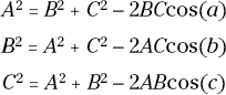
The parallelogram method is a basic geometric method for determining the resultant of two vectors by constructing a parallelogram. You locate the resultant force and then use the laws of sines and cosines to perform calculations on one half (a triangular section) of the parallelogram. A parallelogram is a specific variation of the quadrilateral (four-sided geometric shape) and is shown in Figure 7-5.
A parallelogram by definition has the following properties:
Opposite sides of the parallelogram are congruent (or equal) and must be parallel.
Opposite angles of the parallelogram are also congruent.
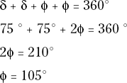
The total sum of the internal angles of a parallelogram must add up to"360 degrees.
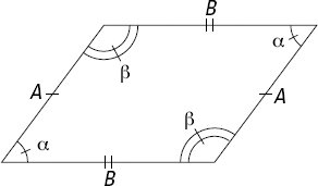
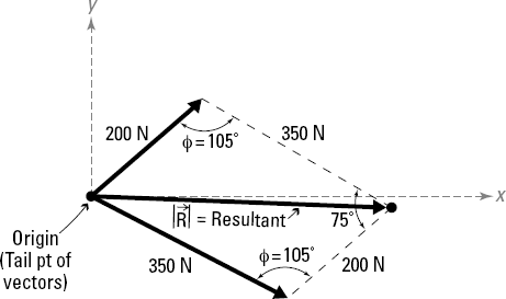
Figure 7-6 shows a block subjected to a force of 200 Newton at an angle of 45 degrees from the vertical, and a second force of 350 Newton at an angle of 30 degrees below the horizontal
To use the parallelogram method, you follow these basic steps:
Connect the two known force vectors at their tail locations, preserving their orientation and magnitude.
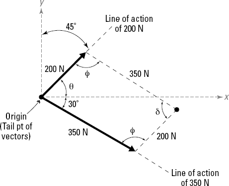
You connect the two vectors at their tails and place this point at the origin of your Cartesian axes as shown in Figure 7-7.
Construct a parallelogram where one side is the magnitude of one of the vectors in its current position and the other side is the magnitude of the other vector in its current position.
In this example, one side of the parallelogram is 200 Newton and the other is 350 Newton, as shown in Figure 7-7. You may have to pick up one of the forces and move it such that the tails of the vector arrows are acting at the same location. You can do that because forces are sliding vectors (or vectors that can act anywhere along their lines of action), so you can actually slide them along their respective lines of action until their tails meet at a common point.
Compute the angle δ between the vectors.
The angle θ is the difference of 90 degrees between the x- and y-Cartesian axes and the 45-degree orientation of the 200-Newton force (so θ = 90° – 45° = 45°). The angle δ is the angle between the 200-Newton and 350-Newton forces and is the sum of θ + 30 degrees, or 75 degrees. Remember that the 30 degrees is the orientation angle of the 350-Newton force below the x-axis.
Compute the angle φ for the remaining angles.
Because you know all quadrilaterals must have a total of 360 degrees in interior angles, you can compute the remaining unknown interior angle as follows:
Draw the resultant force vector as the diagonal of the parallelogram.
Because the parallelogram contains two diagonals, you select the one that shares the tail points of the original vector. In this example, the tail of the resultant is at the same point as the tail of the original 200-Newton and 350-Newton vectors, and the head of the resultant is at the opposite corner, as you can see in Figure 7-8).
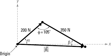
Remove one of the triangular regions from the parallelogram that was created when you sketched the resultant force vector in Step 5.
Which triangle you select makes no difference because they're both the same. The top triangle has the same angles and sides as the bottom one. Include any dimensional or angular information that you may know or have previously calculated. In Figure 7-9, I've chosen the upper triangle for my calculations in this example.
Use the law of cosines to determine the magnitude of the resultant force.
After splitting the parallelogram into a force triangle consisting of the resultant and two sides, you know at least one of the angles of the triangle and the two adjacent sides from the original 200-Newton and 350-Newton vectors. In Figure 7-9, you know two sides of the triangle and the included angle of 105 degrees. You can plug this info into the law of cosines; your result looks something like the following:

Use the law of sines to compute the remaining angle α to help establish the direction of the resultant.
This angle gives the orientation of the resultant relative to the original 200-Newton force vector. At this point, you now know all three side dimensions and one of the related angles. Using the law of sines, you can establish the triangle's ratios.
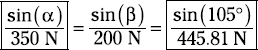
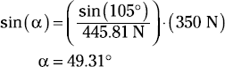
The boxes in this equation just help you remember the pieces you need to solve for. Because you know the 105-degree angle and the opposite side of 445.81 Newton, you can definitely use those two values to establish the ratio. Because you want to compute the angle α, you must use the ratio term that includes that parameter. A bit of rearranging produces the calculation for the desired angle:
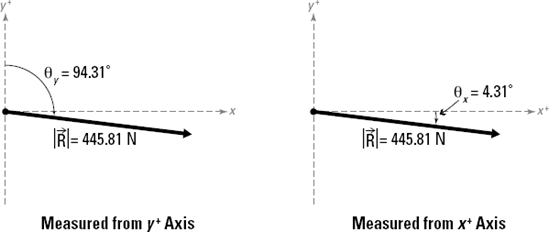
Define your reference line for the angle measurements.
Measuring from the x- or y-axis is usually the most common reference location. However, you can also measure the direction angle of a resultant relative to the angle of any other vector.
If you want to base the calculation from the vertical Cartesian y-axis, you can compute the measured angle from
θy = 45° + 49.31° = 94.31°
which is measured clockwise from the positive Cartesian y-axis. Similarly, if you want to base your reference from the positive Cartesian x-axis, you can report the reference angles as
θx = 90° – θy = 90° – (45° + 49.31°) = −4.31°
In this case, the angle is a negative value, which indicates that it occurs below the positive Cartesian x-axis. Either direction is a correct representation, and both are displayed in Figure 7-10.
One of the most consistent ways of determining a resultant force is by using the vector addition I explore in Chapter 6. You can use this technique with as"many vectors as your heart desires, and it works with two- and three-dimensional problems (unlike the other two techniques in this chapter, which only work easily in two dimensions). It requires only basic math skills — if you can add, you can do vector addition — and it doesn't generally have the accuracy concerns of the graphical techniques (see "Using Graphical Techniques to Construct Resultants" earlier in the chapter). Note: You may need to use some basic trigonometry to create the original vectors in the first place (as I show in Chapter 5), but after that's done, actually computing the resultant is a breeze!
The greatest advantage of the vector methods is that you don't have to find perpendicular distances or worry about maintaining accurate information about the sense of the vector as you do with the other methods in this chapter. All that information is built into the notation of the vector itself. In fact, if you can create vectors, the hardest part of your statics work is already complete because all you need to do is use vector addition to compute the combined result. As long as your calculator has batteries and you can create the necessary Cartesian vectors, finding the resultant vector should be a snap!
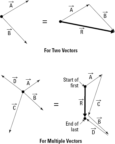
Consider the system of two vectors A and B in Figure 7-11, which shows a simple vector addition case. Vectors A and B are combined to create a resultant vector C. However, with vector addition, you can also find the resultant of multiple vectors all at once. Utilizing the same head-to-tail construction technique I discuss in the graphical methods section earlier in this chapter, you can quickly determine the resultant for the system. However, if you know the vector representation for each of the forces A, B, C, and D, you can find the resultant as being from the tail of vector A to the head of vector D.
If you have the vectors defined in vector notation with all the i, j, and k pieces already determined (see Chapter 5), you can calculate resultants with the following vector addition formula:
Even better, you can expand this simple example to easily handle multiple vectors in exactly the same way:
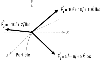
Consider the example of Figure 7-12, which shows a particle subjected to three forces F1, F2, and F3.
To find the resultant of these vectors, you simply add them together:
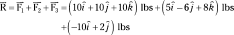
Gathering all of the terms in front of i, j, and k, you can then simplify the expression to
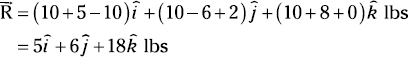
Thus, the resultant of the three vectors of this example is 5i + 6j + 18k, which itself is in vector notation. From here, you can then find the magnitude of the vector by using the following equation:
After you've computed the vector form and the magnitude of the resultant, you can define the direction in any of the ways I define in Chapter 5. Perhaps the easiest is to simply create a unit vector from this information. For the example in the preceding section, you need to divide the resultant vector by its magnitude to create the unit vector that describes the direction. You can then compute the direction cosines to determine the angles if you so desire. The following equation shows you how to create a unit vector for Figure 7-12 in the previous section.