11 Multivariate Normal Examples, Ignoring the Missingness Mechanism
11.1 Introduction
In this chapter, we apply the tools of Part II to a variety of common problems involving incomplete data on multivariate normally distributed variables: estimation of the mean vector and covariance matrix; estimation of these quantities when there are restrictions on the mean and covariance matrix; multiple linear regression, including analysis of variance (ANOVA), and multivariate regression; repeated measures models, including random coefficient regression models where the coefficients themselves are regarded for maximum likelihood (ML) computations as missing data; and selected time series models. Robust estimation with missing data is discussed in Chapter 12, the analysis of partially-observed categorical data is considered in Chapter 13, and the analysis of mixed continuous and categorical data is considered in Chapter 14. Chapter 15 concerns models with data missing not at random.
11.2 Inference for a Mean Vector and Covariance Matrix with Missing Data Under Normality
Many multivariate statistical analyses, including multiple linear regression, principal components analysis, discriminant analysis, and canonical correlation analysis, are based on the initial summary of the data matrix into the sample mean and covariance matrix of the variables. Thus inference for the population mean and covariance matrix for an arbitrary pattern of missing values is a particularly important problem. In Sections 11.2.1 and 11.2.2 we discuss ML for the mean and covariance matrix from an incomplete multivariate normal sample, assuming the missingness mechanism is ignorable. Section 11.2.3 describes Bayesian inference and multiple imputation (MI) for this problem. Although the assumption of multivariate normality may appear restrictive, the methods discussed here can provide consistent estimates under weaker assumptions about the underlying distribution. The multivariate normality assumption will be relaxed somewhat when we consider linear regression in Section 11.4 and robust estimation in Chapter 12.
11.2.1 The EM Algorithm for Incomplete Multivariate Normal Samples
Suppose that (Y1, Y2,…, YK) have a K-variate normal distribution with mean μ = (μ1,…, μK) and covariance matrix Σ = (σjk). We write Y = (Y(0), Y(1)), where Y represents a random sample of size n on (Y1,…, YK), Y(0) the set of observed values, and Y(1) the missing data. Also, let y(0),i represent the set of variables with values observed for unit i, i = 1,…, n. The loglikelihood based on the observed data is then
(11.1)
where μ(0),i and Σ(0),i are the mean and covariance matrix of the observed components of Y for unit i.
To derive the expectation–maximization (EM) algorithm for maximizing (11.1), we note that the hypothetical complete data Y belong to the regular exponential family (8.19) with sufficient statistics
At the tth iteration of EM, let θ(t) = (μ(t), Σ(t)) denote current estimates of the parameters. The E step of the algorithm for iteration t + 1 calculates
(11.2)
and
(11.3)
where
(11.4)
and
(11.5)
Missing values yij are thus replaced by the conditional mean of yij given the set of values, y(0),i observed for that unit and the current estimates of the parameters, θ(t). These conditional means and the nonzero conditional covariances are easily found from the current parameter estimates by sweeping the augmented covariance matrix so that the variables y(0),i are predictors in the regression equation and the remaining variables y(1),i are outcome variables. The sweep operator is described in Section 7.4.3. Note that Eqs. (11.2) and (11.4) impute the best linear predictors of the missing values given current estimates of the parameters, thus showing the link between ML and efficient imputation of the missing values. Equation (11.3) includes adjustments cjki needed to correct for biases in the resulting estimated covariance matrix from imputing conditional means for the missing values.
The M step of the EM algorithm is straightforward. The new estimates θ(t+1) of the parameters are computed from the estimated complete-data sufficient statistics. That is,
(11.6)
Beale and Little (1975) suggest replacing the factor n−1 in the estimate of σjk by (n − 1)−1, which parallels the correction for degrees of freedom in the complete-data case.
It remains to suggest initial values of the parameters. Four straightforward possibilities are (i) to use the complete-case solution of Section 3.2; (ii) to use one of the available-case (AC) solutions of Section 3.4; (iii) to form the sample mean and covariance matrix of the data filled in by one of the single-imputation methods of Chapter 4; or (iv) to form means and variances from observed values of each variable and set all starting correlations equal to zero. Option (i) provides consistent estimates of the parameters if the data are missing completely at random (MCAR) and there are at least K + 1 complete observations. Option (ii) makes use of all the available data but can yield an estimated covariance matrix that is not positive definite, leading to possible problems in the first iteration. Options (iii) and (iv) generally yield inconsistent estimates of the covariance matrix, but estimates that are either positive semidefinite (Option iii) or positive definite (Option iv), and hence are usually workable as starting values. A computer program for general use should have several alternative initializations of the parameters available so that a suitable choice can be made. Another reason for having a variety of starting values available is to examine the likelihood for multiple maxima.
Orchard and Woodbury (1972) first described this EM algorithm. Earlier, the scoring algorithm for this problem had been described by Trawinski and Bargmann (1964) and Hartley and Hocking (1971). An important difference between scoring and EM is that the former algorithm requires inversion of the information matrix of μ and Σ at each iteration. After convergence, this matrix provides an estimate of the asymptotic covariance matrix of the ML estimates, which is not needed by, nor obtained by, the EM computations. The inversion of the information matrix of θ at each iteration, however, can be expensive because this is a large matrix if the number of variables is large. For the K-variable case, the information matrix of θ has K + K(K + 1)/2 rows and columns, and when K = 30 it has over 100 000 elements. With EM, an asymptotic covariance matrix of θ can be obtained by supplemented expectation–maximization (SEM), bootstrapping, or by just one inversion of the information matrix evaluated at the final ML estimate of θ, as described in Chapter 9.
Three versions of EM can be defined. The first stores the raw data (Beale and Little 1975). The second stores the sums, sums of squares, and sums of cross products for each pattern of missing data (Dempster et al. 1977). Because the version that takes less storage and computation is to be preferred, a preferable option is a third, which mixes the two previous versions, storing raw data for those patterns with fewer than (K + 1)/2 units and storing sufficient statistics for the other more frequent patterns.
11.2.2 Estimated Asymptotic Covariance Matrix of
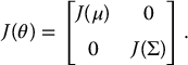
Let θ = (μ, Σ), where Σ is represented as a row vector (σ11, σ12, σ22,…, σKK). If the data are MCAR, the expected information matrix of θ has the form
Here, the ( j, k)th element of J(μ), corresponding to row μj, column μk, is
where
and Σ(0),i is the covariance matrix of the variables observed for unit i. The (ℓm, rs)th element of J(Σ), corresponding to row σℓm, column σrs, is
where δℓm = 1 if ℓ = m, 0 if ℓ ≠ m. As noted earlier, the inverse of supplies an estimated covariance matrix for the ML estimate The matrix J(θ) is estimated and inverted at each step of the scoring algorithm. Note that the expected information matrix is block diagonal with respect to the means and the covariances. Hence, if these asymptotic variances are only required for ML estimates of means or linear combinations of means, then it is only necessary to calculate and invert the information matrix J(μ) corresponding to the means, which has relatively small dimension.
The observed information matrix, which is calculated and inverted at each iteration of the Newton–Raphson algorithm, is not even block diagonal with respect to μ and Σ, so this complete-data simplification does not occur. On the other hand, the standard errors based on the observed information matrix can be viewed as valid when the data are missing at random (MAR) but not MCAR, and hence, should be preferable to those based on J(θ) in applications. For more discussion, see Kenward and Molenberghs (1998). As noted above, EM does not yield an information matrix, so if any such matrix is used as a basis for standard errors, it must be calculated and inverted after the ML estimates are obtained, as with SEM described in Section 9.2.1. A simple alternativewith sufficient data is to compute the ML estimates on bootstrap samples, and apply the methods of Section 9.2.2.
11.2.3 Bayes Inference and Multiple Imputation for the Normal Model
We now describe a Bayesian analysis of the multivariate normal model in Section 11.2.1. To simplify the description, we assume the conventional Jeffreys' prior distribution for the mean and covariance matrix:
and present an iterative data augmentation (DA) algorithm for generating draws from the posterior distribution of θ = (μ, Σ):
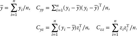
where ℓ(μ, Σ ∣ Y(0)) is the loglikelihood in Eq. (11.1). Let θ(t) = (μ(t), Σ(t)) and denote current draws of the parameters and filled-in data matrix at iteration t. The I step of the DA algorithm simulates
Because the rows of the data matrix Y are conditionally independent given θ, this is equivalent to drawing
(11.7)
independently for i = 1,…, n. As noted in the discussion of EM, this distribution is multivariate normal with mean given by the linear regression of y(1),i on y(0),i, evaluated at current draws θ(t) of the parameters. The regression parameters and residual covariance matrix of this normal distribution are obtained computationally by sweeping on the augmented covariance matrix
so that the observed variables are swept in (conditioned on) and the missing variables are swept out (being predicted). The draw is simply obtained by adding to the conditional mean in the E step of EM, Eqs. (11.2) and (11.4), a normal draw with mean 0 and a function of the current draw of the covariance matrix of the missing variables given the observed variables in unit i, say .
The P step of DA draws
where is the imputed data from st the I step (11.7). The draw of θ(t+1) can be accomplished in two steps:
(11.8)
where is the sample mean and covariance matrix of Y from the imputed data Y(t+1). The posterior distribution of θ can be simulated directly using Eqs. (11.7) and (11.8), after a suitable burn-in period to achieve stationary draws. For more computational details on the P step, see Example 6.19.
An alternative analysis is MI, which creates sets of draws of the missing data based on Eq. (11.7), and then derives inferences using the MI combining rules given in Section 10.2. The Chained Equation algorithm discussed in Section 10.2.4, with normal linear additive regressions for the conditional distributions of each variable given the others, provides an alternative to the DA algorithm. It also yields draws from the predictive distribution of the missing values that can be used to create MI data sets, although (as usually implemented) the predictive distributions are slightly different because of different choices of prior distributions for the parameters of the conditional distributions.
Example 11.1St. Louis Risk Research Data. We illustrate these methods using data in Table 11.1 from the St. Louis Risk Research Project. One objective of the project was to evaluate the effects of parental psychological disorders on various aspects of the development of their children. Data on n = 69 families with two children were collected. Families were classified according to risk group of the parent (G), a trichotomy defined as follows:
(G = 1), a normal group of control families from the local community.
(G = 2), a moderate-risk group where one parent was diagnosed as having secondary schizo-affective or other psychiatric illness or where one parent had a chronic physical illness.
(G = 3), a high-risk group where one parent had been diagnosed as having schizophrenia or an affective mental disorder.
Table 11.1 Example 11.1, St. Louis risk research data
Low risk (G = 1)
Moderate risk (G = 2)
High risk (G = 3)
First child
Second child
First child
Second child
First child
Second child
R1
V1
D1
R2
V2
D2
R1
V1
D1
R2
V2
D2
R1
V1
D1
R2
V2
D2
110
?
?
?
150
1
088
085
2
076
078
?
098
110
?
112
103
2
118
165
1
?
130
2
?
098
?
114
133
?
127
138
1
092
118
1
116
145
2
114
125
?
108
103
2
090
100
2
113
?
?
?
?
?
?
?
?
126
?
?
113
?
2
095
115
2
107
093
?
092
075
?
118
140
1
118
123
?
?
065
?
097
068
2
?
?
1
101
?
2
?
120
?
105
128
?
118
?
2
?
?
2
?
?
?
087
098
2
?
?
?
096
113
?
092
?
2
?
?
?
114
?
2
?
?
2
138
163
1
130
140
?
090
?
1
110
?
2
056
058
2
088
105
1
115
153
1
?
?
?
098
123
?
096
088
?
096
095
1
087
100
2
?
145
2
139
185
2
113
110
?
112
115
?
126
135
2
118
133
?
126
138
1
105
133
1
102
130
?
114
120
?
?
?
?
130
195
?
120
160
?
109
150
?
089
113
2
130
135
?
?
?
?
116
?
2
?
133
?
098
108
?
090
080
2
091
075
2
064
045
2
082
053
2
?
?
?
115
140
2
?
?
?
109
088
2
128
?
2
121
?
2
115
158
2
?
135
1
075
063
1
088
013
1
?
120
1
108
118
?
112
115
2
093
140
?
093
?
I
?
?
?
?
?
?
100
140
2
133
168
1
126
158
2
?
?
?
115
?
2
105
138
1
074
075
1
118
180
1
116
148
?
123
170
1
115
138
2
088
118
?
084
103
?
123
?
1
110
155
1
114
130
2
104
123
2
100
?
1
101
120
1
?
?
2
113
123
2
118
138
1
?
110
1
113
?
2
?
?
2
103
108
?
?
?
?
117
?
?
082
103
2
121
155
1
?
100
2
122
?
1
114
?
2
?
?
?
?
?
2
105
?
2
?
?
1
?
?
?
104
118
1
?
?
?
087
085
1
?
?
?
?
063
?
? denotes missing.
In this example, we compare data on K = 4 continuous variables R1, V1, R2 and V2 by risk group G, where Rc and Vc are standardized reading and verbal comprehension scores for the cth child in a family, c = 1, 2. The variable G is always observed, but the outcome variables are missing in a variety of different combinations, as seen in Table 11.1. Analysis of two categorical outcome variables D1 = number of symptoms for first child (1, low; 2, high) and D2 = number of symptoms for second child (1, low; 2, high) in Table 11.1 is deferred until Chapter 13.
Table 11.2 displays estimates for the four continuous outcomes in the low-risk group and the combined moderate and high-risk groups. The columns show estimates of the mean, standard error of the mean (sem), and the standard deviation from four methods: AC analysis, ML with sem computed using the bootstrap, DA with estimates and standard errors based on 1000 draws of the posterior distribution, and MI based on 10 MI's and the formulae in Section 10.2. Estimates from DA and MI yield very similar results, as expected, and ML is generally similar. The results from AC analysis are broadly similar, but the estimated means deviate noticeably in some cases, namely V1 and R2 for the low risk group, and V1 and V2 for the moderate/high risk groups. General conclusions of superiority cannot be inferred without knowing the true estimand values, but the ML, DA, and MI estimates appear to make better use of the observed data.
Table 11.2 Example 11.1, means and SD's of continuous outcomes in low-, medium-, and high-risk groups, St. Louis risk research data
Low risk (G = 1)
Moderate- and high-risk (G = 2, 3)
Variable
Mean
sem
SD
Mean
sem
SD
V1
AC
146.1
4.8
19.7
105.5
6.6
30.8
ML
143.4
5.5
19.5
115.7
5.9
31.8
DA
143.7
5.4
22.7
115.6
6.3
34.3
MI
143.8
5.4
22.5
115.6
6.3
34.4
V2
AC
128.6
5.4
25.9
106.6
5.4
28.9
ML
128.6
5.1
25.7
110.8
5.1
27.8
DA
128.5
6.0
28.6
110.6
5.2
30.0
MI
128.5
6.0
28.6
110.8
5.2
30.0
R1
AC
117.9
2.3
09.4
102.7
3.2
17.7
ML
116.8
2.9
10.0
103.4
3.3
18.1
DA
116.8
2.8
12.2
103.4
3.4
19.5
MI
116.8
2.8
12.2
103.3
3.3
19.5
R2
AC
110.7
3.2
13.7
101.6
2.5
15.0
ML
108.1
3.0
13.8
101.9
2.5
14.6
DA
108.5
3.4
15.4
101.8
2.7
15.7
MI
108.4
3.4
15.4
101.8
2.7
15.7
Estimates from available-case analysis (AC), maximum likelihood (ML), data augmentation (DA), and multiple imputation (MI), under normal model.
The Bayesian analysis readily provides inferences for other parameters. For example, substantive interest concerns the comparison of means between risk groups. Figure 11.1 shows plots of the posterior distributions of the differences in means for each of the four outcomes, based on 9000 draws. The posterior distributions appear to be fairly normal. The 95% posterior probability intervals based on the 2.5th–97.5th percentiles are shown below the plots. The fact that three of these four intervals are entirely positive is evidence that reading and verbal means are higher in the low-risk group than in the moderate- and high-risk group.
Figure 11.1 Example 11.1, posterior distributions of mean differences μlow − μmed/high, St. Louis risk research data, based on 9000 draws.
11.3 The Normal Model with a Restricted Covariance Matrix
In Section 11.2, there were no restrictions on the parameters of the multivariate normal, θ being free to vary anywhere in its natural parameter space. Many important statistical models, however, place restrictions on θ. ML and Bayes for such restricted models with incomplete data can be readily handled, whenever the complete-data analyses subject to the restrictions are simple. The reason is that the E step of EM, or the I step of DA, take the same form whether θ is restricted or not; the only changes are to modify the M step of EM or the P step of DA to be appropriate for the restricted model.
For some kinds of restrictions on θ, noniterative ML or Bayes estimates do not exist even with complete data. In some of these cases, EM or DA can be used to compute ML or Bayes estimates by creating fully missing variables in such a way that the M or P step is noniterative. We present EM algorithms for two examples to illustrate this idea. Both examples can be easily modified to handle missing data among the variables with some observed values.
Example 11.2Patterned Covariance Matrices. Some patterned covariance matrices that do not have explicit ML estimates can be viewed as submatrices of larger patterned covariance matrices that do have explicit ML estimates. In such a case, the smaller covariance matrix, say Σ11, can be viewed as the covariance matrix for observed variables and the larger covariance matrix, say Σ, can be viewed as the covariance matrix for both observed and fully missing variables. In such a case, the EM algorithm can be used to calculate the desired ML estimates for the original problem, as described by Rubin and Szatrowski (1982).
As an illustration, suppose that we have a random sample y1,…, yn from a multivariate normal distribution, N3(0, Σ11), with the 3 × 3 stationary covariance pattern
The ML estimate of Σ11 does not have an explicit form. However, these observations can be viewed as the first three of four components from a random sample ( y1, z1),…, ( yn, zn) from a multivariate normal distribution N4(0, Σ), where
If ( yi, zi) are all observed, ML estimates of Σ can be computed by simple averaging (Szatrowski 1978). Thus, we apply the EM algorithm, assuming the first three components of each ( yi, zi) are observed, and the last component, zi, is missing. The { yi} are the observed data, and the ( yi, zi) are the complete data, both observed and missing. Let C = ∑ ( yi, zi)T( yi, zi)/n and The matrix C is the complete-data sufficient statistic and C11 is the observed sufficient statistic.
There is only one pattern of incomplete data (yi observed and zi missing), so the E step of the EM algorithm involves calculating the expected value of C given the observed sufficient statistic C11 and the current estimate Σ(t) of Σ, namely, C(t) = E(C ∣ C11, Σ(t)). First, find the regression parameters of the conditional distribution of zi given yi by sweeping Y from the current estimate of Σ, Σ(t), to obtain
The expected value of zi given the observed data and so that the expected value of given C11 and Σ(t) is The expected value of given the observed data and Σ = Σ(t) is
so that the expected value of is
These calculations are summarized as follows:
(11.9)
The ML estimate of Σ given the complete data, C, is explicit and as noted above is obtained by simple averaging. Thus, the M step of EM at iteration t + 1 is given by
(11.10)
where is the (k,j)th element of C(t+1), the expected value of C from the E step (11.9) at iteration t + 1. These estimates of θ1, θ2, and θ3 yield a new estimate of Σ for iteration t + 1. This new value of C is used in (11.10) to calculate new estimates of θ1, θ2, and θ3 and thus Σ(t+1).
An advantage of EM is its ability to handle simultaneously both missing values in the data matrix and patterned covariance matrices, both of which occur frequently in a variety of applications, such as educational testing examples. In some of these examples, unrestricted covariance matrices do not have unique ML estimates because of the missing data, and the patterned structure is easily justified from theoretical considerations and from empirical evidence on related data (Holland and Wightman 1982; Rubin and Szatrowski 1982). When there is more than one pattern of incomplete data, the E step computes expected sufficient statistics for each of the patterns rather than just one pattern as in (11.9).
Example 11.3Exploratory Factor Analysis. Let Y be an n × K observed data matrix and Z be an n × q unobserved “factor-score matrix,” q < K, and let ( yi, zi) denote the ith row of (Y, Z). Assume
(11.11)
where β (K × q) is commonly called the factor-loading matrix, Iq is the (q × q) identity matrix, is called the uniquenesses matrix, and θ = (μ, β, Σ). Integrating out the unobserved factors zi yields the exploratory factor-analysis model:
In factor analysis, it is often assumed that μ = 0; the slightly more general model (11.11) leads to centering the variables Y by subtracting the sample mean for each variable. Little and Rubin (1987) present an EM algorithm for ML estimation of θ. Here we present the faster ML algorithm of Rubin and Thayer (1982), which Liu et al. (1998) show to be an example of a Parameter-expanded expectation–maximization (PX-EM) algorithm.
As discussed in Section 8.5.3, PX-EM creates a model in a larger parameter space where the fraction of missing information is reduced. The expanded model is
(11.12)
where φ = (μ*, β*, Σ*, Γ), and the unrestricted covariance matrix Γ replaces the identity matrix Iq in (11.11). Under model (11.12), ( yi ∣ φ) ∼indNK(μ*, β*Γβ*T + Σ*), so
where Chol(Γ) is the Cholesky factor of Γ (see Example 6.19). The complete data sufficient statistics for (11.12) (that is, if {( yi, zi), i = 1,…, n} were fully observed), are
Given current parameter estimates φ(t), the E step of PX-EM consists of computing the expected complete-data sufficient statistics:
where γ(t) and are the regression coefficients and residual covariance matrix of Z on Y given φ(t). Specifically, let
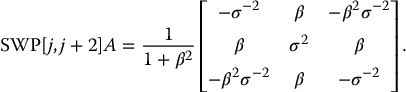
be the current variance–covariance matrix of (Y, Z); then γ(t) and are obtained from the last q columns of SWP[1,…, K] B(t).
The M step of PX-EM calculates the cross-products matrix
It then sets , , and finds β*(t+1) and Σ*(t+1) from the last q columns of SWP[1,…, K] C(t+1). Reduction to the original parameters θ gives μ(t+1) = μ*(t+1), Σ(t+1) = Σ*(t+1), and β(t+1) = β*(t+1)Chol(Γ(t+1)).
This EM algorithm for factor analysis can be extended to handle missing data Y(1) in the Y variables, by treating both Y(1) and Z as missing data. The E step then calculates the contribution to the expected sufficient statistics from each pattern of incomplete data, rather than just the single pattern with yi completely observed.
Example 11.4Variance Component Models. A large collection of patterned covariance matrices arises from variance components models, also called random effects or mixed effects ANOVA models. The EM algorithm can be used to obtain ML estimates of variance components and more generally covariance components (Dempster et al. 1977; Dempster et al. 1981). The following example is taken from Snedecor and Cochran (1967, p. 290).
In a study of artificial insemination of cows, semen samples from K = 6 bulls were tested for their ability to conceive, where the number, ni, of semen samples tested from bulls varied from bull to bull; the data are given in Table 11.3. Interest focuses on the variability of the bull effects; that is, if an infinite number of samples had been taken from each bull, the variance of the six resulting means would be calculated and used to estimate the variance of the bull effects in the population. Thus, with the actual data, there is one component of variability due to sampling bulls from a population of bulls, which is of primary interest, and another due to samples from each bull.
Percentages of conception to services for successive samples
ni
Xi
1
46, 31, 37, 62, 30
5
206
2
70, 59
2
129
3
52, 44, 57, 40, 67, 64, 70
7
394
4
47, 21, 70, 46, 14
5
198
5
42, 64, 50, 69, 77, 81, 87
7
470
6
35, 68, 59, 38, 57, 76, 57, 29, 60
9
479
Total
350
18760
A common normal model for such data is
(11.13)
where are the between-bull effects, are the within-bull effects, and are fixed parameters. Integrating over the αi, the yij are jointly normal with common mean μ, common variance and covariance within the same bull and 0 between bulls. That is
where ρ is commonly called the intraclass correlation.
Treating the unobserved random variables α1,…, α6 as missing data (with all yij observed) leads to an EM algorithm for obtaining ML estimates of θ. Specifically, the complete-data likelihood has two factors, the first corresponding to the distribution of yij given αi and θ, and the second to the distribution of αi given θ:
The resulting loglikelihood is linear in the following complete-data sufficient statistics:
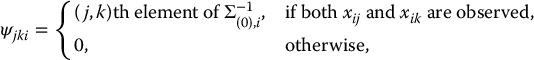
The E step of EM takes the expectations of T1, T2, T3 given current estimates of θ and the observed data yij, i = 1,…, K, j = 1,…, ni. These follow by applying Bayes's theorem to the joint distribution of the αi and the yij to obtain the conditional distribution of the αi given the yij:
where and . Hence,
(11.14)
The ML estimates based on complete data are
(11.15)
Thus, the M step of EM replaces Tj by in these expressions, for j = 1,…, 3.
ML estimates from this algorithm are
, , and . The latter two estimates can be compared with , , obtained by equating observed and expected mean squares from a random-effects ANOVA (e.g., see Brownlee 1965, section 11.4). Far more complex variance-components models can be fit using EM including those with multivariate yij, αi, and X variables; see, e.g., Dempster et al. (1981) and Laird and Ware (1982). Gelfand et al. (1990) consider Bayesian inference for normal random effects models.
11.4 Multiple Linear Regression
11.4.1 Linear Regression with Missingness Confined to the Dependent Variable
Suppose a scalar outcome variable Y is regressed on p predictor variables X1,…, Xp and missing values are confined to Y. If the missingness mechanism is ignorable, the incomplete observations do not contain information about the regression parameters, . Nevertheless, the EM algorithm can be applied to all observations and will obtain iteratively the same ML estimates as would have been obtained noniteratively using only the complete observations. Somewhat surprisingly, it may be easier to find these ML estimates iteratively by EM than noniteratively.
Example 11.5Missing Outcomes in ANOVA. In designed experiments, the set of values of (X1,…, Xp) is chosen to simplify the computation of least squares estimates. When Y given (X1,…, Xp) is normal, least squares computations yield ML estimates. When values of Y, say yi, i = 1,…, m, are missing, the remaining complete observations no longer have the balance occurring in the original design with the result that ML (least squares) estimation is more complicated. For a variety of reasons given in Chapter 2, it can be desirable to retain all observations and treat the problem as one with missing data.
When EM is applied to this problem, the M step corresponds to the least squares analysis on the original design and the E step involves finding the expected values and expected squared values of the missing yi's given the current estimated parameters :
where X is the (n × p) matrix of X values. Let Y be the (n × 1) vector of Y values, and Y(t+1) the vector Y with missing components yi replaced by estimates from the E step at iteration t + 1. The M step calculates
(11.16)
and
(11.17)
The algorithm can be simplified by noting that Eq. (11.16) does not involve and that at convergence we have
Consequently, the EM iterations can omit the M step estimation of and the E step estimation of and find by iteration. After convergence, we can calculate directly from (11.18). These iterations, which fill in the missing data, re-estimate the missing values from the ANOVA, and so forth, comprise the algorithm of Healy and Westmacott (1956) discussed in Section 2.4.3, with the additional correction for the degrees of freedom when estimating , obtained by replacing n − m in Eq. (11.18) by n − m − p, to obtain the usual unbiased estimate of .
11.4.2 More General Linear Regression Problems with Missing Data
In general, there can be missing values in the predictor variables as well as in the outcome variable. For the moment, assume joint multivariate normality for (Y, X1,…, Xp). Then, applying Property 6.1, ML estimates or draws from the posterior distribution of the parameters of the regression of Y on X1,…, Xp are standard functions of the ML estimates or posterior draws of the parameters of the multivariate normal distribution, discussed in the Section 11.2. Let
(11.19)
denote the augmented covariance matrix corresponding to the variables X1,…, Xp and Xp+1 ≡ Y. The intercept, slopes, and residual variance for the regression of Y on X1,…, Xp are found in the last column of the matrix SWP[1,…, p]θ, where the constant term and the predictor variables have been swept out of the matrix θ. Hence, if is the ML estimate of θ found by the methods of Section 11.2, then ML estimates of the intercept, slopes, and residual variance are found from the last column of Similarly, if θ(d) is a draw from the posterior distribution of θ, then SWP[1,…, p]θ(d) yields a draw from the joint posterior distribution of the intercept, slopes, and residual variance.
Let and be the ML estimates of the regression coefficient of Y on X and residual variance of Y given X, respectively, as found by the EM algorithm just described. These estimates are ML under weaker conditions than multivariate normality of Y and (X1,…, Xp). Specifically, suppose we partition (X1,…, Xp) as (X(A), X(B)), where the variables in X(A) are more observed than both Y and the variables in X(B) in the sense of Section 7.5 that any unit with any observation on Y or X(B) has all variables in X(A) observed. A particularly simple case occurs when X = (X1,…, Xp) is fully observed so that X(A) = X: see Figure 7.1 for the general case, where Y1 corresponds to (Y, X(B)) and Y3 corresponds to X(A) and Y2 is null. Then and are also ML estimates if the conditional distribution of (Y, X(B)) given X(A) is multivariate normal – see Chapter 7 for details. This conditional multivariate normal assumption is much less stringent than multivariate normality for X1,…, Xp+1, because it allows the predictors in X(A) to be categorical variables, as in “dummy variable regression,” and also allows interactions and polynomials in the completely observed predictors to be introduced into the regression without affecting the propriety of the incomplete data procedure. Similarly for Bayesian inference, if are draws from the posterior distribution from multivariate normal DA algorithm, they are also draws from the posterior distribution under a conditional multivariate normal model for (Y, X(B)) given X(A).
The (p × p) submatrix of the first p rows and columns of does not provide the asymptotic covariance matrix of the estimated regression coefficients, as is the case with complete data. The asymptotic covariance matrix of the estimated slopes based on the usual large-sample approximation generally involves the inversion of the full information matrix of the means, variances, and covariances, which is displayed in Section 11.2.2. Computationally, simpler alternatives are to apply the bootstrap, or to simulate the posterior distribution of the parameters. In particular, the set of draws SWP[1,…, p]θ(d), where θ(d) is a draw from the posterior distribution of θ, can be used to simulate the posterior distribution of SWP[1,…, p]θ, thereby allowing the construction of posterior credibility intervals for the regression coefficients and residual variance.
More generally, ML or Bayes estimation for multivariate linear regression can be achieved by applying the algorithms of Section 11.2, and then sweeping the independent variables in the resulting augmented covariance matrix. Specifically, if the dependent variables are Y1,…, YK and the independent variables are X1,…, Xp, then the augmented covariance matrix of the combined set of variables (X1,…, Xp, Y1,…, YK) is estimated using the multivariate normal EM algorithm, and then the variables X1,…, Xp are swept in the matrix. The resulting matrix contains the ML estimates of the (p × K) matrix of regression coefficients of Y on X and the (K × K) residual covariance matrix of Y given X. The parallel operations on draws from the posterior distribution by DA provide draws of the multivariate regression parameters. For a review of these methods and alternatives, see Little (1992).
Example 11.6MANOVA with Missing Data Illustrated Using the St. Louis Data (Example 11.1 Continued). We now apply the multivariate normal model to all the data in Table 11.1, including an indicator variable for the low and medium/high-risk groups, and then sweep the group indicator variable out of the augmented covariance matrix at the final step to yield estimates from the multivariate regression of the continuous outcomes on the group indicator variables. The regression coefficient of the group indicator measures the difference in mean outcome between the low-, medium- and high-risk groups. Figure 11.2 displays histograms of 9000 draws of these regression coefficients from DA. The 95% posterior probability intervals based on the 2.5th–97.5th percentiles are shown in the plots in Figure 11.2. Conclusions are similar to Example 11.1, namely, reading and verbal means appear higher in the low-risk group than in the moderate- and high-risk group.
Figure 11.2 Example 11.6, posterior distributions of mean differences μlow − μmed/high, St. Louis risk research data, based on 9000 draws, multivariate normal regression model.
11.5 A General Repeated-Measures Model with Missing Data
Missing data often occur in longitudinal studies, where subjects are observed at different times and/or under different experimental conditions. Normal models for such data often combine special covariance structures such as those discussed in Section 11.3 with mean structures that relate the mean of the repeated measures to design variables. The following general repeated measures model is given in Jennrich and Schluchter (1986) and builds on earlier work by Harville (1977), Laird and Ware (1982), and Ware (1985). ML for this model has been implemented in a number of software programs, including SAS (1992) and S-Plus (Schafer 1998; Pinheiro and Bates 2000).
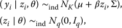
Suppose that the hypothetical complete data for unit i consist of K measurements yi = ( yi1,…, yiK) on an outcome variable Y, and
(11.20)
where Xi is a known (K × m) design matrix for unit i, β is a (m × 1) vector of unknown regression coefficients, and the elements of the covariance matrix Σ are known functions of a set of v unknown parameters ψ. The model thus incorporates a mean structure, defined by the set of design matrices {Xi}, and a covariance structure, defined by the form of the covariance matrix Σ. The observed data consist of the design matrices {Xi} and { y(0),i, i = 1,…, n} where y(0),i is the observed part of the vector yi. Missing values of yi are assumed to be ignorable. The complete-data loglikelihood is linear in the quantities Hence, the E step consists in calculating the means of yi and given y(0),i, Xi, and current estimates of β and Σ. These calculations involve sweep operations on the current estimate of Σ analogous to those in the multivariate normal model of Section 11.2.1. The M step for the model is itself iterative except in special cases, and thus a primary attraction of EM, the simplicity of the M step, is lost. Jennrich and Schluchter (1986) present a generalized EM algorithm (see Section 8.4) and also discuss scoring and Newton–Raphson algorithms that can be attractive when Σ depends on a modest number of parameters, ψ.
A large number of situations can be modeled by combining different choices of mean and covariance structures, for example:
Independence: Σ = DiagK(ψ1,…, ψK), a diagonal (K × K) matrix with entries {ψk},
Compound symmetry: Σ = ψ1UK + ψ2IK, ψ1 and ψ2 scalar, UK = (K × K) matrix of ones, IK = (K × K) identity matrix,
Autoregressive lag 1 (AR1): scalars,
Banded: Σ = (σjk), σjk = ψa, where a = ∣ j − k ∣ + 1,
a = 1,…, K,
Factor analytic: Σ = ΓΓT + ψ, Γ = (K × q) matrix of unknown factor loadings, and ψ= (K × K) diagonal matrix of “specific variances,”
Random effects: Σ = ZψZT + σ2IK, Z = (K × q) known matrix, ψ = (q × q) unknown dispersion matrix, σ2 scalar, IK the K × K identity matrix,
The mean structure is also very flexible. If Xi = IK, then μi = βT for all i. This constant mean structure, combined with the unstructured, factor analytic and compound symmetry covariance structures, yields the models of Section 11.2, Examples 11.3 and 11.4, respectively. Between-subject and within-subject effects are readily modeled through other choices of Xi, as in the next example.
Example 11.7Growth-Curve Models with Missing Data. Potthoff and Roy (1964) present the growth data in Table 11.4 for 11 girls and 16 boys. For each subject, the distance from the center of the pituitary to the maxillary fissure was recorded at the ages of 8, 10, 12, and 14. Jennrich and Schluchter (1986) fit eight repeated-measures models to these data. We fit the same models to the data obtained by deleting the 10 values in parentheses in Table 11.4. The missingness mechanism is designed to be MAR, but not MCAR. Specifically, for both girls and boys, values at age 10 are deleted for cases with low values at age 8. Table 11.5 summarizes the models, giving values of minus twice the loglikelihood (−2λ) and the likelihood ratio chi-squared (χ2) for comparing models. The last column gives values for the latter statistic from the complete data before deletion, as given in Jennrich and Schluchter (1986).
Table 11.4 Example 11.7, growth data for 11 girls and 16 boys
Individual girl
Age (in years)
Individual boy
Age (in years)
8
10
12
14
8
10
12
14
1
21
20
21.5
23
1
26
25
29
31
2
21
21.5
24
25.5
2
21.5
(22.5)
23
26.5
3
20.5
(24)
24.5
26
3
23
22.5
24
27.5
4
23.5
24.5
25
26.5
4
25.5
27.5
26.5
27
5
21.5
23
22.5
23.5
5
20
(23.5)
22.5
26
6
20
(21)
21
22.5
6
24.5
25.5
27
28.5
7
21.5
22.5
23
25
7
22
22
24.5
26.5
8
23
23
23.5
24
8
24
21.5
24.5
25.5
9
20
(21)
22
21.5
9
23
20.5
31
26.0
10
16.5
(19)
19
19.5
100
27.5
28
31
31.5
11
24.5
25
28
28
110
23
23
23.5
25
120
21.5
(23.5)
24
28
130
17
(24.5)
26
29.5
140
22.5
25.5
25.5
26
150
23
24.5
26
30
160
22
(21.5)
23.5
(25)
Values in parentheses are treated as missing in Example 11.6.
Source: Potthoff and Roy (1964) as reported by Jennrich and Schluchter (1986). Reproduced with permission of Oxford University Press.
Eight separate means, unstructured covariance matrix
18,
386.96
—
—
2
Two lines, unequal slopes, unstructured covariance matrix
14,
393.29
1
6.33
4
[2.97]
3
Two lines, common slope, unstructured covariance matrix
13,
397.40
2
4.11
1
[6.68]
4
Two lines, unequal slopes, banded structure
8
398.03
2
4.74
6
[5.17]
5
Two lines, unequal slopes, AR(1) structure
6
409.52
2
16.240
8
[21.20]
6
Two lines, unequal slopes, random slopes and intercepts
8
400.45
2
7.16
6
[8.33]
7
Two lines, unequal slopes, random intercepts (compound symmetry)
6
401.31
2
8.02
8
[9.16]
8
Two lines, unequal slopes, independent observations
5
441.58
7
40.270
1
[50.83]
Source: The complete data is obtained from Jennrich and Schluchter (1986). Reproduced with permission of John Wiley and Sons.
For the ith subject, let yi denote the four distance measurements, and let xi be a design variable equal to 1 if the child is a boy and 0 if the child is a girl. Model 1 specifies a distinct mean for each of the sex by age groups, and assumes that the (4 × 4) covariance matrix is unstructured. The Xi matrix for subject i can be written as
With no missing data, the ML estimate of β is the vector of eight sample means and the ML estimate of Σ is S/n, where S is the pooled within-groups sum of squares and cross-products matrix.
This unrestricted model, Model 1 in Table 11.5, was fitted to the incomplete data of Table 11.4. Seven other models were also fitted to those data. Plots suggest a linear relationship between mean distance and age, with different intercepts and slopes for girls and boys. The mean structure for this model can be written as
(11.21)
where β1 and β1 + β2 represent overall means and β3 and β3 + β4 represent slopes for girls and boys, respectively. Model 2 fits this mean structure with an unstructured Σ.
The likelihood-ratio statistic comparing Model 2 with Model 1 is χ2 = 6.33 on 4 degrees of freedom, indicating a fairly satisfactory fit for Model 2 relative to Model 1. Model 3 is obtained from Model 2 by setting β4 = 0, that is, dropping the last column of Xi. It constrains the regression lines of distance against age to have common slope in the two groups. Compared with Model 2, Model 3 yields a likelihood ratio of 4.11 on 1 degree of freedom, indicating significant lack of fit. Hence, the mean structure of Model 2 is preferred.
The remaining models in Table 11.5 have the mean structure of Model 2, but place constraints on Σ. The autoregressive (Model 5) and independence (Model 8) covariance structures do not fit the data, judging from the chi-squared statistics. The banded structure (Model 4) and two random effects structures (Models 6 and 7) fit the data well. Of these, Model 7 may be preferred on grounds of parsimony. The model can be interpreted as a random effects model with a fixed slope for each sex group and a random intercept that varies across subjects about common means for boys and girls. Further analysis would display the parameter estimates for this preferred model.
11.6 Time Series Models
11.6.1 Introduction
We confine our limited discussion of time-series modeling with missing data to parametric time-domain models with normal disturbances, because these models are most amenable to the ML techniques developed in Chapters 6 and 8. Two classes of models of this type appear particularly important in applications: the autoregressive-moving average (ARMA) models developed by Box and Jenkins (1976), and general state-space or Kalman-filter models, initiated in the engineering literature (Kalman 1960) and enjoying considerable development in the econometrics and statistics literature on time series (Harvey 1981). As discussed in the next section, autoregressive models are relatively easy to fit to incomplete time-series data, with the aid of the EM algorithm. Box–Jenkins models with moving average components are less easily handled, but ML estimation can be achieved by recasting the models as general state-space models, as discussed in Harvey and Phillips (1979) and Jones (1980). The details of this transformation are omitted here; however, ML estimation for general state-space models from incomplete data is outlined in Section 11.6.3, following the approach of Shumway and Stoffer (1982).
11.6.2 Autoregressive Models for Univariate Time Series with Missing Values
Let Y = ( y0, y1,…, yT) denote a completely observed univariate time series with T + 1 observations. The autoregressive model of lag p (ARp) assumes that yi, the value at time i, is related to values at p previous time points by the model
(11.22)
where θ = (α, β1, β2,…, βp, σ2), α is a constant term, β1, β2,…, βp are unknown regression coefficients, and σ2 is an unknown error variance. Least squares estimates of α, β1, β2,…, βp and σ2 can be found by regressing yi on xi = ( yi−1, yi−2,…, yi−p), using observations i = p, p + 1,…, T. These estimates are only approximately ML because the contribution of the marginal distribution of y0, y1,…, yp−1 to the likelihood is ignored, which is justified when p is small compared with T.
If some observations in the series are missing, one might consider applying the methods of Section 11.4 for regression with missing values. This approach may yield useful rough approximations, but the procedure is not ML, even assuming the marginal distribution of y0, y1,…, yp−1 can be ignored, because (i) missing values yi (i ≥ p) appear as dependent and independent variables in the regressions, and (ii) the model (11.22) induces a special structure on the mean vector and covariance matrix of Y that is not used in the analysis. Thus, special EM algorithms are required to estimate the ARp model from incomplete time series. The algorithms are relatively easy to implement, although not trivial to describe. We confine attention here to the p = 1 case.
Example 11.8The Autoregressive Lag 1 (AR1) Model for Time Series with Missing Values. Setting p = 1 in Eq. (11.22), we obtain the model
(11.23)
The AR1 series is stationary, yielding a constant marginal distribution of yi over time, only if |β| < 1. The joint distribution of the yi then has constant marginal mean μ ≡ α(1 − β)−1, variance Var( yi) = σ2(1 − β2)−1, and covariances Cov( yi, yi+k) = βkσ2(1 − β2)−1 for k ≥ 1. Ignoring the contribution of the marginal distribution of y0, the complete-data loglikelihood for Y is which is equivalent to the loglikelihood for the normal linear regression of yi on xi = yi−1, with data {( yi, xi), i = 1,…, T}. The complete-data sufficient statistics are s = (s1, s2, s3, s4, s5), where
ML estimates of θ = (α, β, σ) are where
(11.24)
Now suppose some observations are missing, and missingness is ignorable. ML estimates of θ, still ignoring the contribution of the marginal distribution of y0 to the likelihood, can be obtained by the EM algorithm. Let θ(t) = (α(t), β(t), σ(t)) be estimates of θ at iteration t. The M step of the algorithm calculates θ(t+1) from Eq. (11.24) with complete data sufficient statistics s replaced by estimates s(t) from the E step.
The E step computes where
and
The E step involves standard sweep operations on the covariance matrix of the observations. However, this (T × T) matrix is usually large, so it is desirable to exploit properties of the AR1 model to simplify the E step computations. Suppose is a sequence of missing values between observed values yj and yk. Then (i) is independent of the other missing values, given Y(0) and θ, and (ii) the distribution of given Y(0) and θ depends on Y(0) only through the bounding observations yj and yk. The latter distribution is multivariate normal, with constant covariance matrix, and means that are weighted averages of μ = α(1 − β)−1, yj and yk. The weights and covariance matrix depend only on the number of missing values in the sequence and can be found from the current estimate of the covariance matrix of ( yj, yj+1,…, yk) by sweeping on elements corresponding to the observed variables yj and yk.
In particular, suppose yj and yj+2 are present and yj+1 is missing. The covariance matrix of yj, yj+1 and yj+2 is
Substituting θ = θ(t) in these expressions yields and for the E step.
11.6.3 Kalman Filter Models
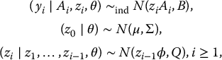
Shumway and Stoffer (1982) consider the Kalman filter model
(11.26)
where yi is a (1 × q) vector of observed variables at time i, Ai is a known (p × q) matrix that relates the mean of yi to an unobserved (1 × p) stochastic vector zi, and θ = (B, μ, Σ, φ, Q) represents the unknown parameters, where B, Σ, and Q are covariance matrices, μ is the mean of z0, and φ is a (p × p) matrix of autoregression coefficients of zi on zi−1. The random unobserved series zi, which is modeled as a first-order multivariate autoregressive process, is of primary interest.
This model can be envisioned as a kind of random effects model for time series, where the effect vector zi has correlation structure over time. The primary aim is to predict the unobserved series {zi} for i = 1, 2,…, n (smoothing) and for i = n + 1, n + 2,… (forecasting), using the observed series y1, y2,…, yn. If the parameter θ were known, the standard estimates of zi would be their conditional means, given the parameters θ and the data Y. These quantities are called Kalman smoothing estimators, and the set of recursive formulas used to derive them are called the Kalman filter. In practice, θ is unknown, and the forecasting and smoothing procedures involve ML estimation of θ, and then application of the Kalman filter with θ replaced by the ML estimate
The same process applies when data Y are incomplete, with Y replaced by its observed component, say Y(0). ML estimates of Q can be derived by Newton–Raphson techniques (Gupta and Mehra 1974; Ledolter 1979; Goodrich and Caines 1979). However, the EM algorithm provides a convenient alternative method, with the missing components Y(1) of Y and z1, z2,…, zn treated as missing data. An attractive feature of this approach is that the E step of the algorithm includes the calculation of the expected value of zi given Y(0) and current estimates of θ, which is the same process as Kalman smoothing described above. Details of the E step are given in Shumway and Stoffer (1982). The M step is relatively straightforward. Estimates of φ and Q are obtained by autoregression applied to the expected values of the complete data sufficient statistics
from the E step; B is estimated by the expected value of the residual covariance matrix Finally, μ is estimated as the expected value of z0, and Σ is set from external considerations. We now provide a specific example of this very general model.
Example 11.9A Bivariate Time Series Measuring an Underlying Series with Error. Table 11.6, taken from Meltzer et al. (1980), shows two incomplete time series of total expenditures for physician services, measured by the Social Security Administration (SSA), yielding Y1, and the Health Care Financing Administration (HCFA), yielding Y2. Shumway and Stoffer (1982) analyze the data using the model
where yij is the total expenditure amount at time i for SSA ( j = 1) and HCFA ( j = 2), zi is the underlying true expenditure, assumed to form an AR1 series over time with coefficient φ and residual variance Q,Bj is the measurement variance of yij ( j = 1, 2), and θ = (B1, B2, φ, Q). Unlike Example 11.8, the AR1 series for zi is not assumed stationary, the parameter φ being an inflation factor modeling exponential growth; the assumption that φ is constant over time is probably an oversimplification. The last columns of Table 11.6 show smoothed estimates of zi from the final iteration of the EM algorithm for years 1949–1976, and predictions for the five years 1977–1981, together with their standard errors. The predictions for 1977–1981 have standard errors ranging from 355 for 1977 to 952 for 1982, reflecting considerable uncertainty.
Table 11.6 Example 11.9, data set and predictions from the EM algorithm – physician expenditures (in millions)
SSA
HCFA
Predictions from EM algorithm
Year (i)
yi1
yi2
E(zi ∣ Y(0), θ)
Var1/2(zi ∣ Y(0), θ)
1949
2 633
—
2 541
178
1950
2 747
—
2 711
185
1951
2 868
—
2 864
186
1952
3 042
—
3 045
186
1953
3 278
—
3 269
186
1954
3 574
—
3 519
186
1955
3 689
—
3 736
186
1956
4 067
—
4 063
186
1957
4 419
—
4 433
186
1958
4 910
—
4 876
186
1959
5 481
—
5 331
186
1960
5 684
—
5 644
186
1961
5 895
—
5 972
186
1962
6 498
—
6 477
186
1963
6 891
—
7 032
185
1964
8 065
—
7 866
179
1965
8 745
8 474
8 521
110
1966
9 156
9 175
9 198
108
1967
10 2870
10 1420
10 1600
108
1968
11 0990
11 1040
11 1590
108
1969
12 6290
12 6480
12 6450
108
1970
14 3060
14 3400
14 2890
108
1971
15 8350
15 9180
15 8350
108
1972
16 9160
17 1620
17 1710
108
1973
18 2000
19 2780
19 1060
109
1974
—
21 5680
21 6750
119
1975
—
25 1810
25 0270
120
1976
—
27 9310
27 9320
129
1977
—
31 1780
355
1978
—
34 8010
512
1979
—
38 8460
657
1980
—
43 3610
802
1981
—
48 4000
952
Source: Meltzer et al. (1980) as reported in Shumway and Stoffer (1982), Tables I and III. Reproduced with permission of John Wiley and Sons.
11.7 Measurement Error Formulated as Missing Data
In Chapter 1, we described how measurement error can be formulated as a missing-data problem, where the true values of a variable measured with error are treated as completely missing. Guo and Little (2011) apply this idea to internal calibration data with heteroskedastic measurement error. In our final example in this chapter, we describe MI to address measurement error for data from a main sample and an external calibration sample, described in Example 1.15. For more details, see Guo et al. (2011).
Example 11.10Measurement Error as Missing Data: A Normal Model for External Calibration. In Example 1.15, we described data displayed in Figure 11.3, where the main sample data are a random sample of values of U and W, where W is the proxy variable for X, and information relating W and X is obtained from an external calibration sample in which values of X and W are recorded. Here X and W are univariate, U is a vector of p variables, and interest concerns parameters of the joint distribution of X and U. The missingness pattern is similar to that of the file-matching problem described in Example 1.7. An important special case is where U = (Y, Z), where Y is a vector of q outcomes, Z is a vector of r covariates, p = q + r, and interest lies in the regression of Y on Z and X. This pattern arises in the case of external calibration, where calibration of W is carried out independently of the main study, for example by an assay conducted by the manufacturer. Typically, data from the calibration sample are not available to the analyst, but we assume that summary statistics – namely the mean and covariance matrix of X and W – are available. We assume the missing data, namely the values of X in the main sample, and the missing values of Y and Z in the calibration sample, are ignorable.
Figure 11.3 Missingness pattern for Example 11.10, with shaded values observed. X = true covariate, missing in the main sample; W = measured covariate, observed in both the main and calibration samples; U = other variables, missing in the calibration sample.
Guo et al. (2011) assume that in the main sample and the calibration sample, the conditional distribution of U and X given W is (p + 1)-variate normal with a mean that is linear in W and a constant covariance matrix. Further, this conditional distribution is assumed to be the same in the main study sample and the calibration sample, although the distribution of W can differ in the two samples. This indispensable assumption is a form of the “transportability across studies” assumption in Carroll et al. (2006). It is evident from Figure 11.3 that the joint distribution cannot be estimated from the data without invoking more assumptions, because the variables X and U are never jointly observed. Specifically, there is no information about the p partial correlations of X and U given Z.
To address this issue, we make the “nondifferential measurement error” (NDME) assumption, which states that the distribution of U given W and X does not depend on W.
This assumption is reasonable if the measurement error in W is unrelated to values of U = (Y, Z), and is plausible in some bioassays. Our approach multiply-imputes the missing values of X in the main study from the estimated conditional distribution of X given the observed variables in the main study sample, namely U and W; under normality assumptions, this is surprisingly straightforward, computationally. Let θx⋅uw = (βx⋅uw, σx⋅uw) where βx⋅uw denotes the vector of regression coefficients and σx⋅uw the residual standard deviation for that regression. For data set d, a draw is taken from the posterior distribution of θx⋅uw. This draw can be computed rather simply from the main sample data and summary statistics from the external calibration sample, namely the sample size, sample mean and sum of squares and cross products matrix of X and W.
Specifically, let θ = (βxw⋅w, σxx⋅w, βuw⋅w, σuu⋅w, σux·w), where (βxw⋅w, σxx⋅w) are the regression coefficients and residual variance for the (normal) regression of X on W, (βuw⋅w, σuu⋅w) are the regression coefficients and residual covariance matrix for the (normal) regression of U on W, and σux·w represents the set of p partial covariances of U and X given W. Now:
Draw from the distribution of (βuw⋅w, σuu⋅w), given the data on U and W in the main study sample; and
Draw from the distribution of (βxw⋅w, σxx⋅w), given the data on X and W in the calibration sample. Note that these draws can be computed from summary statistics in the calibration sample, namely the sample size, sample mean, and sum of squares and cross-products matrix of X and W.
Both (a) and (b) are straightforward, because both these distributions are posterior distributions for complete-data problems, as discussed in Example 6.17. To obtain a draw for the remaining component of θ, namely σux·w, note that by properties of the normal distribution, the regression coefficient of W in the multivariate regression of U on X and W can be expressed as
The NDME assumption implies that βuw⋅xw = 0. Hence
Thus we have expressed σux·w as a function of the other parameters, and a draw of σux·w is:
(11.27)
Combining, we thus have a draw from the conditional distribution of X and U given W. Missing values xi of X for the ith observation in the study sample are then imputed as draws from the conditional normal distribution of X given U and W, with parameters and , functions of θ(d), obtained by sweeping out U to convert U from dependent to independent variables. That is
where is the conditional mean of xi given ( yi, zi, wi), the values of (Y, Z, W) for unit i, is the residual variance of the distribution of X given U and W, and is a draw from the standard normal distribution. This method is proper in the sense discussed in Chapter 10, because it takes into account uncertainty in estimating the parameters.
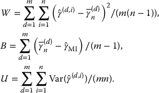
The external calibration data are not generally available in the postimputation analysis. Reiter (2008) shows that in this situation, the standard MI combining rules in Chapter 10 yield a positively biased estimate of sampling variance, and resulting confidence interval coverage exceeds the nominal rate. Reiter (2008) describes an alternative two-stage imputation procedure to generate imputations that lead to consistent estimation of sampling variances. Specifically, we first draw d values of model parameters φ(d); second, for each φ(d), d = 1,…, m, we construct n imputed data sets by generating n sets of draws of X. The resulting m × n imputed datasets are then analyzed by the following combining rules:
For d = 1,…, m and i = 1,…, n, let and be the estimated parameters of interest and the associated estimated sampling variance computed with D(d, i) data set, respectively. The MI estimate of γ, γMI, and associated sampling variance TMI are calculated as
where
The 95% interval for γ is , with degrees of freedom
When TMI < 0, the sampling variance estimator is recalculated as (1 + 1/m)B, and inferences are based on a t-distribution with (m − 1) degrees of freedom.
Problems
Show that the available-case estimates of the means and variances of an incomplete multivariate sample, discussed in Section 3.4, are ML when the data are specified as multivariate normal with unrestricted means and variances, and zero correlations, with ignorable nonresponse. (This result implies that the available-cases method works reasonably well when the correlations are low.)
Write a computer program for the EM algorithm for bivariate normal data with an arbitrary pattern of missing values.
Write a computer program for generating draws from the posterior distribution of the parameters, for bivariate normal data with an arbitrary pattern of missing values, and a noninformative prior for the parameters.
Describe the EM algorithm for bivariate normal data with means (μ1, μ2), correlation ρ, and common variance σ2, and an arbitrary pattern of missing values. If you did Problem 11.2, modify the program you wrote to handle this model. (Hint: For the M step, transform to U1 = Y1 + Y2, U2 = Y1 − Y2.)
Derive the expression for the expected information matrix in Section 11.2.2, for the special case of bivariate data.
For bivariate data, find the ML estimate of the correlation ρ for (a) a bivariate sample of size r, with known means (μ1, μ2) and known variances , and (b) a bivariate sample of size r, and effectively infinite supplemental samples from the marginal distributions of both variables. Note the rather surprising fact that (a) and (b) yield different answers.
Prove the statement before Eq. (11.9) that complete-data ML estimates of Σ are obtained from C by simple averaging. (Hint: Consider the covariance matrix of the four variables U1 = Y1 + Y2 + Y3 + Y4, U2 = Y1 − Y2 + Y3 − Y4, U3 = Y1 − Y3, and U4 = Y2 − Y4.)
Review the discussion in Rubin and Thayer (1978, 1982) and Bentler and Tanaka (1983) on EM for factor analysis.
Derive the EM algorithm for the model of Example 11.4 extended with the specification that μ ∼ N(0, τ2), where μ is treated as missing data. Then consider the case where τ2 → ∞, yielding a flat prior on μ.
Examine Beale and Little's (1975) approximate method for estimating the covariance matrix of estimated slopes in Section 11.4.2, for a single predictor X, and data with (a) Y completely observed and X subject to missing values, and (b) X completely observed and Y subject to missing values. Does the method produce the correct asymptotic covariance matrix in either case?
Fill in the details leading to the expressions for the mean and variance of yj+1 given yj, yj+2, and θ in Example 11.8. Comment on the form of the expected values of yj+1 as β ↑ 1 and β ↓ 0.
For Example 11.8, extend the results of Problem 11.11 to compute the means, variances, and covariance of yj+1 and yj+2 given yj, yj+3 and θ, for a sequence where yj and yj+3 are observed, and yj+1 and yj+2 are missing.
Develop a Gibbs' sampler for simulating the posterior distributions of the parameters and predictions of the {zi} for Example 11.9. Compare the posterior distributions for the predictions for years 1949 and 1981 with the EM predictions in the last two columns of Table 11.6.