CHAPTER 5
BASIC CONCEPTS OF PROBABILITY
LEARNING OBJECTIVES
• Understand initial concepts and definitions associated with the basic concepts of probability
• Understand and apply the principles associated with marginal probabilities, joint probabilities, and conditional probabilities
• Understand the definition of and concepts associated with binomial probability
• Understand the definition of the Poisson distribution and how it is different from a binomial distribution
• Understand the definition of the normal distribution and how it differs from the Poisson and binomial distributions
All statistics are based on probability. Probability is just a formal way of referring to chance. If, for example, we were to flip a coin, we would know that there is some chance that it will come up heads and, by implication, some chance that it will come up tails. We know, in general, that this chance is fifty-fifty for either heads or tails occurring. But we also know that there is no certainty at all to the way the coin will come up. If the coin is flipped in what any of us would think of as the normally appropriate way, we are pretty sure that the resulting head or tail will have come up totally by chance or, in statistical terms, randomly. This random occurrence of heads or tails makes the result of a coin flip conform to what statisticians call a stochastic process. Simply put, a stochastic process is one for which any result has a certain probability of occurrence. In this case, the probability of any result of the flip of a single coin (either heads or tails) is 0.5.
5.1 SOME INITIAL CONCEPTS AND DEFINITIONS
Any discussion of probability requires agreement on some initial concepts and definitions. The following sections provide working definitions for probability concepts.
All statistics are based on probability. Probability is a formal way of talking about chance. Therefore, we need probability to help us link chance and statistics.
Events, Independent Events, Outcomes, and Sample Space
An observation to which a probability can be assigned is often referred to as an event. If we flip a coin, we might reasonably think of that as an event (that is, the flip). But in this chapter we will actually think of the event as the viewing of the results of the flip. To understand how we will consider this, think of the story of the three umpires—the traditionalist, the pragmatist, and the existentialist. The traditionalist umpire, in calling balls and strikes, says, “I call ’em as they are.” The pragmatist says, “I call ’em as I see ’em.” The existentialist says, “They ain’t nothin’ until I call ’em.” We will take the existentialist view. The result of a coin flip is nothing until we view it and “call” the result.
An event is defined as an observation to which a probability can be assigned.
Independent Events If we flip a coin twice, it is generally assumed that the outcome of the first flip will have no bearing on the outcome of the second flip. The first event does not influence the second event in any way. In statistical terms, it is said that the two events (flip one and flip two) are independent of each other. When we flip the coin the first time, the probability of our getting either a head or a tail is 0.5. When we flip the coin the second time, the probability of either a head or a tail is again 0.5. There are four possible outcomes of the flip of two coins: HH, HT, TH, or TT. The probability of any one of these four outcomes is 0.25, because each is equally likely and one divided by four is 0.25. But we can also arrive at the probability of any one of these four outcomes by the rule that says the probability of any outcome of two independent events is the multiplication of the probability of each separate event. Thus, the probability of the outcome HH is 0.5 times 0.5, which is 0.25, which is also the probability of the outcome TH, HT, or TT. This rule is referred to as the simple multiplication rule.
In general we will talk of individual observations as events and the accumulation of those observations as outcomes. However, a single event—the flip of a coin that results in a tail—may also be considered an outcome if there is only one coin flip.
Just in passing, it might be interesting to think about what the multiplication of probabilities of independent events may mean for long sequences of coin flips. If we were told that a person had flipped a coin five times and gotten the sequence HTTHT, we would not be particularly surprised. But if we were told that the person had gotten the sequence HHHHH, we would perhaps question the accuracy of the reporting or the honesty of the reporter. But the probability of either of these two outcomes as the result of five flips of a coin is exactly the same: 0.5 × 0.5 × 0.5 × 0.5 × 0.5, or 0.55, or 0.03125.
Why, then, are we not surprised by the first outcome but are surprised by the second? The answer lies in the fact that we would expect the result of five flips of a coin to include some heads and some tails, even though we would not necessarily expect any particular order of heads and tails. When we see a specific ordering that includes both heads and tails, our expectation is confirmed without our recognizing that the specific ordering we see is no more likely than five heads in a row.
Sample Space The two possible outcomes from the flip of a coin—heads or tails—are frequently called the sample space for this process. The sample space refers to all the possible outcomes of a particular process. The sample space for two flips of a coin includes the outcomes HH, HT, TH, and TT. For five flips of a coin, the sample space includes 25, or thirty-two, separate outcomes. As we have seen, each of these individual outcomes has the same probability (0.03125) of occurring. But it is often less the specific outcome than the mix of heads and tails that will interest us in the flip of five coins.
“Sample space” refers to all the possible outcomes of a particular process.
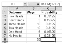
From the perspective of the mix of heads and tails, the outcomes of five flips of a coin include five heads, four heads and one tail, three heads and two tails, two heads and three tails, one head and four tails, and five tails. There is only one way that an outcome of five heads can occur—if each flip is a head. The outcome of four heads and one tail can occur five ways. For example, the first four flips could come up heads and the last a tail; or there could be three heads, a tail, and then a head or two heads, then a tail, and then two heads, and so on. There are actually ten ways that the results could be three heads and two tails, ten ways to get two heads and three tails, five ways to get one head, and one way to get no heads (all tails).
FIGURE 5.1 Possible combinations of five coin flips
Mutually Exclusive Outcomes
Figure 5.1 shows the thirty-two ways that the five flips of a coin can come out in terms of the number of heads realized. As the table shows, there is one way to obtain five heads, five ways to obtain four heads, and so on. In five flips of a coin, each of the thirty-two outcomes is mutually exclusive of all others. Being mutually exclusive means, for example, that the result HHHHH and the result HTTHT cannot both occur. One can occur or the other can occur, but the occurrence of one precludes the occurrence of the other (and, similarly, all other outcomes).
Mutual exclusivity means that only one event in a sample space can occur at a time.
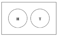
A Venn diagram uses circles to represent sets, with the position and overlap (if any) of the circles indicating the relationships between the sets. Figure 5.2 displays a Venn diagram for two events that are mutually exclusive. For our coin example, there are two circles. One circle represents heads, H, and one circle represents tails, T. Notice in Figure 5.2 that the two circles do not overlap. In the context of a Venn diagram, this illustrates that the two events, heads and tails, are mutually exclusive.
When outcomes are mutually exclusive, their probabilities can be summed. For example, there are five ways in which four heads can occur, each of the ways having a probability of 0.03125. The sum of these five ways is the total probability of getting four heads in any one of the five ways, which is shown in Figure 5.1 as 0.15625. The probability of getting three heads or two heads is given in Figure 5.1 as 0.3125, which is the sum of the probability of getting any combination of either three or two heads. The probabilities of all mutually exclusive outcomes in the sample space must add to 1. This is considered one of the rules of probability.
FIGURE 5.2 Venn diagram for two mutually exclusive events
The discussion of Figure 5.1 allows us to better understand why we would probably not be surprised by a sequence of HTTHT from the flip of five coins, whereas we would be surprised by the sequence HHHHH. The probability of seeing two heads and three tails from five flips of a coin is 0.3125, almost one-third. In looking at the sequence HTTHT, we ignore the specific pattern and think only of the combination of heads and tails. The probability of seeing five heads, however, is only 0.03125, or about three chances out of one hundred. Consequently, we would be much more surprised to see that result. Be careful not to confuse the concept of independence and the concept of mutual exclusivity. Think of independence when you have successive events (e.g., two flips of a coin) and think of mutual exclusivity when you think of events in the event space (e.g., in any one flip I can obtain a head or a tail, but not both at the same time).
A Priori Probability and Empirical Probability
There are two types of probability to consider. The first of these is the probability associated with the flip of a coin or, for example, with the roll of a die or the draw of a card from a deck. The nature of the object or objects upon which the random process is based determines the probability of the outcome. The probability of the outcome of a head after the flip of a coin is 0.5 given the nature of the coin (it has only two sides). The probability that a two will come up on the roll of a fair six-sided die is approximately 0.1667 (1/6) given the nature of the die. The probability of drawing an ace from the top of a well-shuffled deck is approximately 0.0769 (4/52) given the nature of the deck of cards (there are four aces in a fifty-two-card deck). This type of probability is called a priori probability. Virtually all games of chance are based on a priori probabilities.
A priori probabilities are objective and are known “a priori” or before the event has occurred.
The second type of probability is probability associated with a set of objects about which we do not have the necessary knowledge to specify a probability a priori. These probabilities are referred to as subjective probabilities or probabilities that are random in nature. For example, if we were to consider people arriving for treatment at a hospital emergency room, they could be divided into two types: those who are coming for true emergencies, however defined, and those coming for nonemergency conditions. If we are interested in the probability that the next person arriving at the emergency room will have a true emergency, we cannot generally call upon some a priori knowledge of the people arriving and the propensity for their conditions to be emergencies or nonemergencies in determining that probability.
Subjective probabilities are random in nature and thus not known before the occurrence of an event.
Frequency of Occurrence and Empirical Probability What we can rely on to gauge this probability of occurrence is some historical record of persons arriving at the emergency room. Suppose we have a record of all the arrivals at the emergency room for the past six months, during which time there were 7,320 total emergency room visits (about forty per day). We also have information about whether the visit was for a true emergency as assessed by the attending physician, physician’s assistant, or nurse. Suppose the record indicates that 4,729 of the visits were true emergencies. Now we can say that for the past six months, the probability that a person coming to the emergency room came for a true emergency was 0.646 (4,729/7,320). Based on this, and assuming that the future is like the past, we could predict that when the next person arrives at the clinic, that person has about a 0.65 probability of having a true emergency and about a 0.35 probability of having a nonemergency problem. This type of probability is known as empirical probability.
An empirical probability is one based on actual observations or event occurrences.
To consider another example of empirical probability, suppose we have records on 2,556 married women, and for each of these women we have recorded the number of children born to that woman. Thinking back to the definition of event that was given in the first subsection of Section 5.1, the recording of the number of children born to each woman is the event. The distribution of women by number of children born might look something like Figure 5.3. This table shows that 256 of the women have had no children born, 682 have had one child, 796 have had two children, and so on. Among these 2,556 women, no woman has had more than seven children born.
Figure 5.3 also shows the proportion of women with no children, one child, two children, and so on. This proportion also represents an empirical probability. In this case, it is the empirical probability that any woman drawn at random from our group of 2,556 will have no children, or one child, and so on. For example, the empirical probability that a woman drawn at random from among the 2,556 would have four children is 0.0865. The probability that a woman drawn at random would have no children is 0.1001. The other probabilities follow similarly.
FIGURE 5.3 Children ever born to 2,556 women
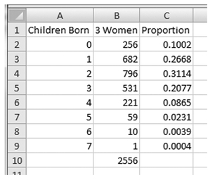
If our 2,556 women had been a random sample from some larger population, we would be able to ascribe the probabilities associated with numbers of children to that larger population as well. In particular, if we were to select another woman from that larger population, we would be able to anticipate that the probability was about 0.0004 that the woman selected would have seven children, based on the empirical probabilities for our 2,556 women. Similarly, we would be able to say that the probability was about 0.2076 that she would have three children, again based on the empirical probabilities.
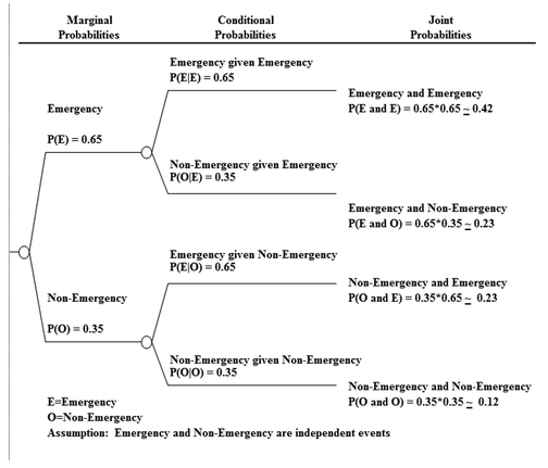
Sequential Events and Empirical Probabilities Empirical probabilities work just like a priori probabilities in regard to sequential events. For example, if we looked at the record of the sequential arrival of any two people at the emergency room, we would see four possible events. If we classify true emergencies as E and nonemergency conditions as O (other), then the results of the arrival of two sequential people could be EE, EO, OE, and OO. Now, however, despite the fact that there are four possible outcomes, the probability of each outcome is not 0.25. If we do assume for the moment that the outcome of the arrival of the first person (that is, E or O) does not influence the outcome of the arrival of the second person, then we can say that the arrival outcomes are independent of one another. Under the assumption of independence, the probability that the outcome will be EE is 0.65 × 0.65, or 0.42. The probability of EO is 0.65 × 0.35, or 0.23. The probability of the outcome OE is the same as that of EO, and the probability of the outcome OO is 0.35 × 0.35, or 0.12. Because these four mutually exclusive outcomes represent the entire sample space, the reader can confirm that the probabilities for the four sum to 1. Figure 5.4 displays the probability tree associated with emergency and nonemergency situations. Per the probability tree, marginal probabilities are listed first, followed by conditional probabilities and finally joint probabilities.
FIGURE 5.4 Sequential events
Independence and Empirical Probabilities With empirical probabilities, though, unlike the case with a priori probabilities, we may not always be justified in viewing many events as independent. It is likely that several persons arriving at an emergency room in a sequential manner may be dependent on one another in regard to their emergency or nonemergency status. If, for example, there occurred a large highway accident that sent a number of persons to emergency rooms, several persons arriving at the same time might all be related (and hence not independent) emergencies. In fact, one of the most important capabilities of statistics is the ability to assess whether events are independent of or dependent on one another. The concept of independence is one that we will return to over and over in the course of this book.
Empirical Probability and Probability Distributions In many instances, data of interest to health workers can be viewed only from the standpoint of empirical probability. Whether an arrival at an emergency room is an emergency or not can be understood only as an empirical probability. But, interestingly, once we know what the overall probability of being an emergency is, and if we assume that the arrival of an emergency is independent of whether the last person arriving was an emergency, we can apply a priori probability assumptions to the arrival of several people at a time. In other words, those arrivals could be modeled using a probability distribution, and the a priori assumption we apply is that those arrivals are from a binomial distribution. The binomial distribution is discussed in detail later in this chapter. In fact, numerous distributions can be used to model data depending on the specific character or shape of the data. Another very important distribution is the normal distribution. The normal distribution is important in that one of the most important assumptions for statistics is that both discrete numerical data and continuous numerical data will somehow follow, a priori, a normal distribution. Normal distributions are discussed further in this chapter, and also in chapter six.

EXERCISES FOR SECTION 5.1
1. Calculate the probability of the following:
a. The sequential roll of the die faces 2, 4, and 3
b. The sequence of coin flips HTHH
c. Assuming a probability of any arrival at an emergency room being an emergency as 0.646, and assuming that arrivals are independent, the probability of the next four arrivals’ being all emergencies
d. Assuming (c), the probability of the next five arrivals’ being all nonemergencies
e. Assuming (c), the probability of the next four arrivals’ being two emergencies and two nonemergencies, in that order
f. Assuming a probability of 0.5 that any child born will be a boy, the probability of any family of five children having no girls
2. Lay out on a Microsoft Excel spreadsheet the possible outcomes of two rolls of a fair die and calculate the following:
a. The probability that the two faces of the dice will equal 7
b. The probability that the two faces of the dice will equal 11
c. The probability that the two faces of the dice will equal 8 or more
3. Lay out on an Excel spreadsheet the possible outcomes of a visit by three persons to an emergency room. Assuming that the visits are independent, with a probability of 0.646 of being an emergency, calculate the following:
a. The probability of two emergencies out of three arrivals
b. The probability of no emergencies out of three arrivals
c. The probability of at least two emergencies out of three arrivals
5.2 MARGINAL PROBABILITIES, JOINT PROBABILITIES, AND CONDITIONAL PROBABILITIES
To continue with the discussion of probability, it will be useful to distinguish three different types of probabilities: marginal probabilities, joint probabilities, and conditional probabilities. Marginal probabilities are those associated with a single event. “Joint probability” refers to the simultaneous occurrence of two or more types of events. “Joint probabilities” and “conditional probabilities” refer to the outcomes of two different types of events that may or may not be independent of each other.
Marginal probabilities are those associated with a single event. “Joint probability” refers to the simultaneous occurrence of two or more types of events. “Conditional probability” refers to the occurrence of one event given that another event has occurred.
Marginal Probability
The probability (proportion) shown in Figure 5.3 is often referred to as marginal probability . Marginal probability is the probability of the occurrence of a single outcome. The probability that any single woman selected at random from among the 2,556 women will have no children is the number of women with no children divided by the total number of women. “Marginal probability” refers to the probability of an occurrence of any single outcome. By the same token, whether the next person appearing at the emergency room arrives with a true emergency or a nonemergency condition is also a single outcome (or event if we are counting only that one person). The marginal probability for true emergencies, according to the discussion earlier in this chapter, is 0.65, and for nonemergency conditions it is 0.35.
“Marginal probabilities” refers to outcomes that are mutually exclusive of one another. For example, a woman cannot at the same time have no children and three children. These categories are mutually exclusive. Those arriving at an emergency room can be coming either for a true emergency or for a nonemergency condition. In this context, they could not be coming for both. As was noted earlier, the probabilities of mutually exclusive events can be added together. Furthermore, the sum of the probabilities of all possible mutually exclusive marginal probabilities will always be 1. To see the consequences of these two points, consider again Figure 5.3. If we wished to know the probability that a woman would have at least four children, we could add together the probability of any woman’s having four, five, six, and seven children. The resulting probability, 0.1138, is the probability that a woman will have at least four children. In regard to the second point, it is relatively easy to verify that the sum of all probabilities in Figure 5.3 is 1.
Joint Probability
“Marginal probability” refers to the outcome of a single event or type of event (the birth of children, the arrival at an emergency room). “Joint probability” refers to the simultaneous occurrence of two or more types of events. Return to the example of persons arriving at an emergency room. Figure 5.5 shows the first twenty observations in a file that contains records of 7,320 emergency room visits. Column C shows whether the visit was for an emergency or not. Column B is labeled Shift. The first shift (labeled 1st) is from 7 A.M. to 3 P.M. The second shift (labeled 2nd) is from 3 P.M. to midnight, and the third shift (labeled 3rd) is from midnight to 7 A.M.
FIGURE 5.5 First twenty observations in an emergency room visit file
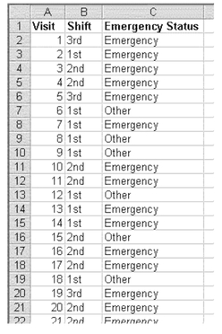
Building a Joint Probability Table Using a Spreadsheet In this example, we might, in addition to determining whether the visit was for a true emergency or a nonemergency condition, determine when during the day the arrival took place. The pivot table option in Excel was used to produce Figure 5.6, which shows the joint occurrence of a true emergency or a nonemergency condition and the shift during which the visit took place. It should be easy to recognize that Figure 5.6 is an example of a contingency table. A contingency table is one that shows the simultaneous occurrence of two or more events. In this case, the events are whether the arrival at the emergency room is or is not an emergency and the shift during which the arrival occurred.
FIGURE 5.6 Contingency table of shift and emergency status
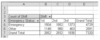
FIGURE 5.7 Joint probabilities for shift and emergency status
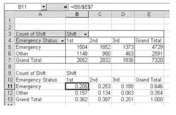
Figure 5.6 shows that of the 4,729 visits that were true emergencies, 1,504 occurred during the first shift, 1,852 occurred during the second shift, and 1,373 occurred during the third shift. Similarly, for visits to the emergency room that were not for true emergencies (the Other category), 1,148 occurred during the first shift, 980 occurred during the second shift, and 463 occurred during the third shift. The probability that, for example, a visit took place during the first shift and was for a true emergency is a joint probability. The joint probability for the simultaneous occurrence of a visit during the first shift and for a true emergency is 1,504/7,320, or 0.205.
Figure 5.7 shows the contingency table for all the joint probability combinations as well as the marginal probabilities for both reason for visit (true emergency or other) and time of day. The calculation of the joint probability is shown in the formula line at the top of the figure. Notice that the dollar sign ($) convention is used to fix the divisor as cell E7 for every internal cell.
The probabilities shown in Figure 5.7 can also be obtained directly from the pivot table capability. In the PivotTable Field dialog box, you can click an Options button (see Figure 4.25). If you click this button, you can then select a “Show Data as” dialog box that allows you to select any one of nine ways to display the data in the pivot table cells. One of these is the normal view, which is given in Figure 5.6. Another is “as percent of the total,” which displays the data as shown in cells A11:E13 of Figure 5.7.
Mutual Exclusivity and the Simple Addition Rule It can be confirmed from the table that the marginal probability (p) that the visit was for a true emergency is equal to the sum of the joint probabilities for the first, second, and third shifts. This can be seen in Equation 5.1. Equation 5.1 is referred to as the simple addition rule. The simple addition rule can be applied here since the first, second, and third shifts are mutually exclusive (i.e., they cannot occur at the same time).

In general, it is always possible to find the marginal probability of occurrence of an event from the joint probabilities of its occurrence when viewed in a contingency table, such as that shown in Figure 5.7. The reader can confirm that the marginal probabilities for the other categories are the sum of the relevant joint probabilities.
Mutual Exclusivity and the Addition Rule Thus far, the discussion has concerned a joint probability that is represented by the conjunction “and.” It is also possible to discuss a joint probability that is represented by the conjunction “or.” The joint probability “or” would be stated in regard to true emergencies and time of day. For example, a visit was for a true emergency or it occurred during the first shift. The joint probability “or” is the sum of the appropriate marginal probabilities minus the appropriate joint probability. At times this is referred to as “avoiding the double count.” We must subtract the joint probability of the two events if those two events are not mutually exclusive. In our example, a visit for a true emergency is not mutually exclusive of time of day. Figure 5.8 is a Venn diagram representing the events from our example, true emergency (TE) and first shift (FS). Notice that the two circles overlap. The overlap represents the intersection of the two events or the joint probability. The overlap indicates that these two events are not mutually exclusive.
Therefore, the probability that a visit was for a true emergency or that it took place during the first shift can be calculated by the formula shown in Equation 5.2.

FIGURE 5.8 Venn diagram of two events that are not mutually exclusive
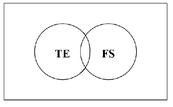
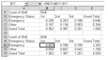
FIGURE 5.9 Joint probability “or” for shift and emergency status
Notice that if we did not subtract the p(True and First), the probability of True or First would be well over 1.0, violating the rules of probability.
Calculating Joint Probability “or” Values in a Spreadsheet Figure 5.9 shows all the joint probability “or” values for arriving during one of three shifts or for coming for an emergency or for a condition that is not an emergency. The formula line shows the calculation of the joint probability p(True or First) as B$13+$E11-B11. This formulation lets us drag the formula in cell B17 to the other five cells and generates the joint probability “or” for each of the cells in the table. The joint probabilities “or” for each row and column have been summed in cells B19:D19 and in cells E17 and E18. At first glance, these numbers mean nothing, because all probability values must be equal to or less than 1 to have meaning. However, the sum of the row probabilities or the sum of the column probabilities can be summed to the total of the joint probabilities “or” in cell E19. For a two-by-three table, such as the one shown in Figure 5.9, the sum of the joint probabilities “or” will always be 4. Four turns out to be the number of rows in the figure plus the number of columns minus 1. In fact, for any contingency table of any size, the sum of all joint probabilities “or” is always equal to the number of rows plus the number of columns minus 1.
It is possible to determine if the calculation of joint probabilities “and” is correct by determining if the probabilities sum to 1. It is equally possible to ensure that the calculation of joint probabilities “or” is correct by determining whether the probabilities sum to the number of rows plus the number of columns minus 1. For example, in a three-by-four table (three rows and four columns), the sum of all joint probabilities “or” would be 3 + 4 - 1, or 6.
Conditional Probability
The discussion of probabilities given thus far has involved the development of probabilities with essentially no prior knowledge of events. The discussion has focused, for example, on the probability that a visit to the emergency room would be for a true emergency and would occur during the first shift. Now the discussion turns to another point of probability—the probability of one event’s occurring if it is known that another event has occurred. For example, suppose we know that an emergency room visit has taken place during the third shift. The task then might be to determine the probability that the visit would be a true emergency, given that it is already known that it took place during the third shift. We might also ask, What is the probability that the visit was an emergency conditional on its having taken place during the third shift? This is known as conditional probability.
Bayes’ Theorem and Conditional Probability The calculation of conditional probabilities can be taken directly from our discussion of marginal and joint probabilities and may be shown as given in Equation 5.3. In Equation 5.3, p(A|B) is read as “the probability of A given B,” which means the probability of A is conditional on B’s having occurred, or having been known. This is also known as Bayes’ Theorem.
In regard to our example of emergency room visits, the conditional probability that a visit was for a true emergency, given that it occurred during the third shift, would be calculated as is shown in Equation 5.4.

The calculation of all the conditional probabilities, given that the arrival took place either during the day or during the night, is shown in Figure 5.10. Cell B17, for example, shows the calculation of the conditional probability that the arrival was for an emergency, given that it took place during the first shift. The formula used for that calculation is =B11/B$13 and is shown in the formula line above the spreadsheet. The formula can be copied into all the cells in the table to calculate the associated conditional probabilities. It is important to note that the conditional probabilities in Figure 5.10 are calculated for the columns. This means that each conditional probability is the probability that the arrival is or is not an emergency, given that it took place during either the first, second, or third shift. Because these probabilities are calculated by column, the total of column conditional probabilities add to 1 for each column. It is also possible to calculate row conditional probabilities. The row conditional probabilities would be interpreted as the probability of coming during a particular shift, given that the visit was for an emergency or not. If conditional probabilities were calculated this way, they would sum to 1 by rows rather than by columns. In general, however, conditional probabilities are usually calculated for columns.
FIGURE 5.10 Conditional probabilities for arrival during any shift
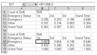
Conditional Probabilities and Data Frequencies Conditional probabilities can also be calculated directly from data frequencies. It should be noted that the conditional probability of the visit to the emergency room being for a true emergency, given that it took place during the first shift, is just the number of visits for true emergencies taking place during the first shift, divided by all the visits taking place during the first shift. If we look at Figure 5.6, for example, we can see that there were 2,652 visits during the first shift, of which 1,504 were for true emergencies. If we divide 1,504 by 2,652, the result is 0.567, which is the same as what we found using the formula in Equation 5.4, or as calculated in Figure 5.10.
Conditional Probability and Independent Events This introduction of the concept of conditional probability provides another opportunity to talk about the notion of independent events and independence. Earlier, independence was defined as being a situation in which the occurrence of one event had no relation to the occurrence of a second event. In particular, if a coin is flipped twice, the second flip is generally assumed to be independent of the first because the result of the first will not influence the result of the second. If the first is a head, we should not expect that a second flip will be any more likely a tail than a head.
The introduction of conditional probability provides another way to look at the independence of events. Two events are independent if all the conditional probabilities of the event are equal to the marginal probabilities of the event. This general relationship is expressed in Equation 5.5. Consider the conditional and marginal probabilities for emergency room visits, shown in Figure 5.10. The conditional probability of a true emergency, given that the visit took place during the first shift, is p(True|First) = 0.567. The marginal probability of a true emergency is p(True) = 0.646. Because these are not equal, arrival for an emergency and arrival during a particular shift are not independent of each other.
The condition of independence, as shown in Equation 5.5, holds for the earlier discussion of the flip of two coins. A first coin, B, is flipped and its outcome is observed (head or tail). For the first flip, the probability of flipping a head, p(HB) = 0.5, or a tail, p(TB) = 0.5. On the second toss, coin A, is flipped and the probability of flipping a head, p(HA) = 0.5, or a tail, p(TA) = 0.5. In fact, there is no difference in the probability of flipping a head or tail on the second coin given the first flip had or had not been observed. Regardless of the results of flip B, the probability of flip A does not change, so p(HA|HB) = p(HA). The previous equation reads: Given that coin B flipped a head, then the probability of coin A flipping a head is simply equal to the marginal probability of coin A flipping a head. This statement illustrates that the events are independent.
This is contrary to our previous example. Considering visits to emergency rooms, the probability that a visit was for a true emergency, given that it took place during the first shift, is p(True|First) = 0.567, but the probability that a visit is a true emergency is p(True) = 0.646. In this case, p(True|First) ≠ p(True) and therefore emergency status and shift are dependent upon each other.
Conditional Probability Tables via Spreadsheet to Test Independence If we had been dealing with a table of two rows and two columns, any conditional probability that did not equal the marginal probability would have forced all conditional probabilities to be different from the marginal probabilities. The nature of a two-by-two table is such that if p(A|B) ≠ p(B) for any individual conditional probability in the table, the principle of independence will hold for all other conditional probabilities in the table. In a table with more than four internal cells, we cannot make that claim.
Consider, again, children ever born to 2,556 women. Suppose these women were divided into low and high income and the number of children ever born were categorized as 0, 1, 2, 3, and 4+, as shown in Figure 5.11. The number of women in the high-and low-income groups, with their respective numbers of children, are shown in cells H2:I5. The column conditional probabilities (the conditional probability, for example, of having 0 children, given that the woman is high income) are given in cells H10:I14. It is possible to see that the conditional probability of having 0 children, given high income (cell H10), is essentially the same as the marginal probability of having no children within three decimal points (cell J10).
FIGURE 5.11 Conditional probabilities for high- and low-income women and number of children
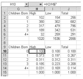
Similarly, the conditional probability of having two children, given high income (cell H12), is the same as the marginal probability of having two children (cell J12). But in other cells, the conditional and marginal probabilities are not equal. For example, the conditional probability of having one child, given high income (cell H11), is not the same as the marginal probability for one child (cell J11). Therefore, it can be concluded that income and number of children born are dependent. It is necessary to show only one occurrence that a conditional probability does not equal a marginal probability to prove dependence.
Mathematical Versus Statistical Independence It is important to point out, however, that the concept of independence discussed thus far is mathematical independence. If Equation 5.5 does not hold, then two events are not mathematically independent. By this definition, the two events, arrival for an emergency and arrival during a particular shift, are not independent. But the conditional probabilities for arrival for an emergency or for a nonemergency condition, given a shift during the day, are not much different from the marginal probabilities. As Figure 5.10 shows, the conditional probability of arriving for an emergency during any particular shift is in every case no more than 0.1 different from the marginal probability. Mathematically speaking they are different; however, viewed another way, are they statistically different? Could we think of those probabilities in terms of statistical independence? The answer to this question is yes. Chapter eight discusses statistical tests for categorical data. These test allow us to determine whether the differences between conditional and marginal probabilities can be considered statistically independent.

EXERCISES FOR SECTION 5.2
1. Use the data in file Chpt 5-2.xls. This is the data file from which the discussion in Section 5.2 was developed. Do the following:
a. Generate a contingency table such as that shown in Figure 5.6, using the pivot table capability of Excel.
b. Calculate the marginal probabilities for both Shift and Emergency Status, as is shown in Figure 5.7.
c. Calculate the joint probabilities “and” for each of the cells in the table, as is shown in Figure 5.7. Confirm that the sum of the cells is 1.
d. Calculate the joint probabilities “or” for each of the cells in the table, as is shown in Figure 5.9. Confirm that the sum of the joint probabilities “or” is equal to rows + columns - 1.
e. Calculate the conditional probabilities of reason for arrival, given that the patient arrives in the first, second, or third shift (replicate Figure 5.10) and confirm that reason for arrival and time of arrival are not independent.
2. Use the file created in Exercise 2 of Section 3.3 of chapter three (or use Chpt 5-3.xls) and do the following:
a. Generate a contingency table with Sex as the column variable and Insurance as the row variable and calculate the marginal probabilities of each variable.
b. Calculate joint probabilities “and” for the two variables and show them in a separate table. Confirm that the joint probabilities “and” sum to 1.
c. Calculate joint probabilities “or” for the two variables and show them in a separate table. Confirm that the joint probabilities “or” sum to rows + columns - 1.
d. Calculate conditional probabilities of having a particular type of insurance, given Sex, and determine if the two variables are independent.
3. Use the file in Exercise 2 (preceding) and do the following:
a. Generate a new variable Charges 2, where Charges 2 is 1 if Charges is greater than the average and 0 if less.
b. Generate a contingency table with Insurance as the column variable and Charges 2 as the row variable and calculate marginal probabilities for each variable.
c. Calculate joint probabilities “and” for the two variables and show them in a separate table. Confirm that the joint probabilities “and” sum to 1.
d. Calculate joint probabilities “or” for the two variables and show them in a separate table. Confirm that the joint probabilities “or” sum to rows + columns - 1.
e. Calculate conditional probabilities for charges, given insurance, and show these in a separate table. Determine if the two variables are independent.
5.3 BINOMIAL PROBABILITY
As has been discussed thus far, a person comes to the emergency room for one of two reasons: either for an emergency or for a nonemergency reason. Because arrival can be for one of two reasons, this can be considered a binary event. The occurrence of binary events generally follows a known distribution, called the binomial distribution. Consider, again, a most common binary event—the flipping of a coin. The result can be either a head or a tail, and either outcome is equally likely (i.e., either outcome has a 0.5 probability of occurrence). But suppose we are flipping the coin five times. Figure 5.1 showed the number of different heads that could be obtained in five flips of a coin. That table indicates that the probability of getting all heads was 0.03125, the probability of getting four heads was 0.15625, the probability of getting three heads was 0.3125, and the probability of getting two one or no heads were exactly the same probabilities in reverse. These probabilities for five flips of a coin follow the binomial distribution.
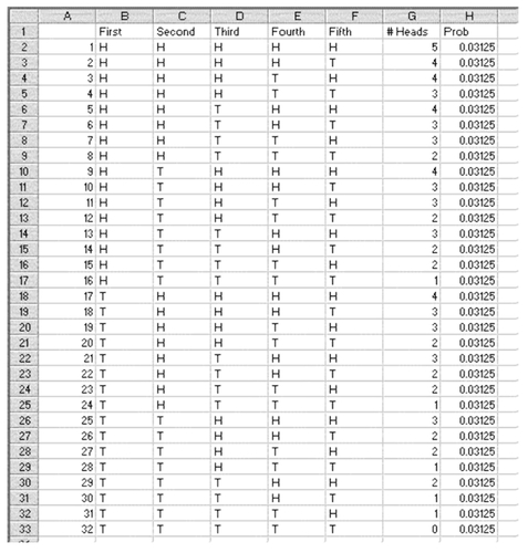
Figure 5.12 shows all the possible outcomes of the flip of a coin five times. Column B shows the result of the first flip, column C shows the result of the second flip, and so on. By examining the figure, it can be seen that there is only one way that the result can be five heads, five ways that the result can be four heads, ten ways that the result can be three heads, and so on, to one way to obtain no heads. The probability of any one of the thirty-two outcomes is given in column H. Each of these outcomes has exactly the same probability: 0.03125. But because there are five ways to get four heads, each of these 0.03125 probabilities can be added together to get the probability of getting four heads. The same can be done for three heads, and so on. The results will be exactly those shown in Figure 5.1.
Applying Binary Logic to Flips of a Coin But is it possible to generalize the information found in Figure 5.12 to any number of coin flips, or, for that matter, to any binary events such as the arrival for an emergency or nonemergency condition? The answer is yes. To do so, let us first consider the probability of getting any number of heads in five flips of the coin. Let us say that we flip a coin five times and we get the outcome HHTHT. This is outcome number six in Figure 5.12. It can then be asked, “What is the probability of getting that outcome?”
The solution is as follows: the probability of a head on the first flip (0.5) times the probability of a head on the second flip (0.5) times the probability of a tail on the third flip (0.5) times the probability of a head on the fourth flip (0.5) times the probability of a tail on the fifth flip (0.5). Because the probabilities of heads or tails are both 0.5, the probability of the outcome HHTHT is 0.5 × 0.5 × 0.5 × 0.5 × 0.5, or 0.55. But it is also the probability of heads raised to the third power times the probability of tails raised to the second power, or 0.53 × 0.52. Think of the number of flips of a coin as being designated by n; think of the occurrence of a head—the outcome we wish to track—as the index value (I) and the number of heads that come up as being designated by x. Then, the probability of any single outcome (that is, of any number of heads in a specific order) in n flips of a coin is given in Equation 5.6.
FIGURE 5.12 All possible outcomes of the flip of a coin five times

where p(I) is the probability of the event I (for example the probability of a head in one flip of a coin) and is the probability of any single outcome of x events in n tries (for example the outcome HHTHT in five flips of a coin). For example, the probability of the specific pattern of heads and tails HHTHT is

Applying Binary Logic to Emergency and Nonemergency Visits For the flip of a coin where the probability of heads and one minus the probability of heads are the same (0.5), the result of Equation 5.6 is exactly the same for any single value of x (that is, for any single number of heads, such as 1 head, 2 heads, and so on). If we consider again the visit of people to an emergency room and use the empirical probabilities shown in Figure 5.6, p(I) and 1—p(I) are not equal (e.g., p(E) = 0.65 and p(O) = 1- 0.65 = 0.35). Consequently, the result of the application of Equation 5.6 will not be the same for every different number of true emergencies (x) and nonemergency conditions. Figure 5.13 shows all the possible outcomes of the visit to an emergency room of five people and their emergency or nonemergency status. We assume that each visit is independent of all other visits. The probability of five emergencies is given as 0.113. You can confirm that this is 0.6465 or p(I)5 × (1 - p(I))(5-5). The equation in cell H2 would resemble this: =(0.646^(G2))*((1-0.646)^(5-G2)). The probability of four emergencies out of five (for example outcome number 2 or outcome number 3) is 0.062. It is possible to confirm that this is 0.6464 × 0.3541 or p(I)4 × (1 - p(I))(5-4), as expressed in Equation 5.6.
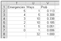
Now that we have calculated the probabilities of occurrence of each of the thirty-two different ways in which five persons can present emergencies or nonemergency conditions in an emergency room, it is possible to add all of the ways that each number of emergencies may be generated to produce the result shown in Figure 5.14. The formula to calculate cell V2 in the column labeled Prob in Figure 5.14 is as follows: =(0.646^(T2))*((1-0.646)^(5-T2))*U2. This formula can then be copied down through cell V7.
Equations for the Binomial Distribution
But there is a less tedious way of getting the result in Figure 5.14 than by enumerating every possible combination. As both Figures 5.13 and 5.14 show, the probability of getting any single number of emergencies is exactly the same for each one of the ways in which that number of emergencies can be obtained. For example, the probability of seeing three emergencies out of five arrivals at the emergency room is 0.034. This is true for any of the ten ways to see three emergencies. Consequently, if there is a way to determine the number of ways that one can find three emergencies out of five visits, it would be possible simply to multiply this number times the probability of finding three emergencies in any single way (Equation 5.6).
Combinatorial Formulas It turns out that there is a formula for finding the number of ways that one can get three emergencies out of five visits. More generally we wish to find x emergencies (I) out of n total observations. That formula is the general formula for the number of combinations out of any number of tries, as is shown in Equation 5.7. Equation 5.7 says that the total number of combinations, (C), for finding n emergencies (I or the Index event) out of n observations is n factorial divided by the quantity x factorial times (n - x) factorial.
FIGURE 5.13 All possible outcomes of five emergency room visits
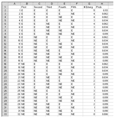
FIGURE 5.14 Probabilities of number of visits that are actual emergencies

where C  is the number of different ways to get x results of I out of n observations. (Three emergencies out of five persons coming to the emergency room, for example.)
Factorials in Excel: The =FACT() Function The term “factorial” means to multiply the number to which the factorial refers by every number less than it in the number sequence. So, for example, 5! is 5 × 4 × 3 × 2 × 1, or 120. The Excel =FACT() function will provide the value of factorials up to 170! (about 7.257E+306 or 7,257 followed by 303 zeros). Now if we wish to know the probability of seeing, for example, x emergencies in the next n persons who come to the clinic, the complete formula is as given in Equation 5.8.

where is the total probability of n results of I out of x observations (the binomial probability).
Figure 5.15 shows the same probabilities as Figure 5.14, except that those in Figure 5.15 were developed using the =FACT() function and the formulas in Equations 5.6, 5.7, and 5.8. Column D in the figure is the result of the application of Equation 5.7. Column E is the result of the application of Equation 5.6. Column F is the binomial probability, which is the result of the application of Equation 5.8. The actual setup of the formulas as implemented in Excel is shown in Figure 5.16. You will recall that the table shown in Figure 5.16 can be generated by going to Tools Options and checking formulas on the View tab.
The formulas for Figure 5.16 were entered only into row 2 and copied to the other rows. It is useful to look closely at Figure 5.16 to see how the $ convention was used to generate the correct cell references in each row.
FIGURE 5.15 Probabilities of number of visits using formulas
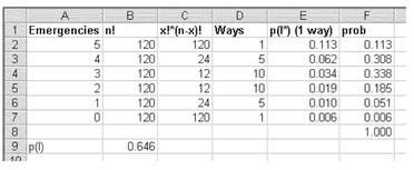
FIGURE 5.16 Formulas used for calculations of probabilities

Binomial Probabilities in Excel: The =BINOMDIST() Function Figure 5.15 was calculated using the formulas in Equations 5.6, 5.7, and 5.8. Excel actually provides a function that produces an easier way to determine binomial probabilities. This is the =BINOMDIST() function. The =BINOMDIST() function takes four arguments. These are the number of emergency visits (5, 4, 3, 2, 1, or 0), the number of visits observed (five), the probability of an emergency (0.646), and a 0 or 1 to indicate whether the value to be determined is the actual probability or the cumulative probability. Figure 5.17 shows the result of using the =BINOMDIST() function to calculate binomial probabilities. The values in column B have been calculated by the formula shown in the formula bar. The values in column C have been calculated by dragging the equation from column B to column C and changing the 0 in the final argument to a 1.
Two additional things should be pointed out. First, the cumulative binomial function always accumulates from the lowest number of the index value (0 emergencies) to the highest. Consequently, column C accumulates from cell C7 to cell C2. Second, it is relatively easy to confirm that the cumulative probabilities are simply the accumulation of the probabilities at each of the number of emergencies. In other words, the cumulative value for two emergencies is the sum of the probabilities for zero emergencies, one emergency, and two emergencies. This seems logical, and it is true because the number of emergencies is a discrete numerical variable. There cannot be a half of an emergency or 3.2 emergencies. We will discuss distributions, particularly the normal distribution (see Section 5.5), where it is not possible to accumulate individual probabilities to get the cumulative probability.
FIGURE 5.17 The =BINOMDIST() function

A final note about Figure 5.17. It is instructive to examine how the $ references have been used to be able to copy the original formula from cell B2 to cells B2:C7 to get all the correct probabilities by changing only the 0 in cell B2 to a 1 in column C.
Binomial Applications to the Health Care Professional To this point there has been ample time spent on the development of the binomial distribution. Therefore it is appropriate to relate the binomial distribution to the health care professional. The binomial distribution can give the probability for the occurrence of any event that can have two outcomes. Let’s continue with emergency room visits example. Suppose a hospital emergency room administrator has data over the past year showing that exactly 20,278 true emergencies were seen in the emergency room out of 31,390 people who sought care from the emergency room. Suppose further that the emergency room administrator is pretty certain that most visits to the emergency room are independent events (i.e., they are not related to one another such as patients from a train wreck or a multiple-car pileup). Using the binomial event logic, the emergency room administrator can figure out how many emergencies she might expect during an eight-hour shift.
She knows from existing data that on any given night on average twenty-nine people will show up at the emergency room. In turn, for staffing purposes she may be interested in the probability that no more than fifteen real emergencies will appear in the emergency room. By using the =BINOMDIST(15,29,0.646,1) function, she will learn that there is a probability of only about 0.106 that fifteen or fewer true emergencies will show up at the emergency room. The administrator would have good reason, then, to be prepared for more than fifteen emergencies, and staff accordingly. Although this is interesting information, the administrator is most likely interested in times when the emergency room is busy.
FIGURE 5.18 Binomial distribution for emergencies in an eight-hour shift
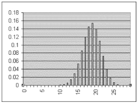
So, for example, what would be the probability that more than twenty-five emergencies would show up during her shift out of the twenty-nine people who come in? That would be found by subtracting =BINOMDIST(25,29,0.646,1) from 1, the result of which is about 0.002. Assuming an eight-hour shift, an occurrence of more than twenty-five emergencies is going to happen only about three times per year. So she would be justified in assuming that only very rarely would she have to be prepared for more than twenty-five true emergencies. Figure 5.18 shows the entire binomial distribution for any number of emergencies (from 0 to 29) occurring during an eight-hour shift. As the figure shows, the administrator can expect between thirteen and twenty-five true emergencies during any eight-hour shift. On virtually no days will the emergency room see fewer than thirteen emergencies and rarely more than twenty-five. This same logic can be applied to any other occurrences that can take on only two values.
Answering the Question of Correctly Documented Medicare Claims In chapter one there is a brief discussion of the problem of incorrectly documented Medicare claims at the Pentad Home Health Agency. The agency drew a random sample of eighty records from their files, and during an audit of the records it was determined that only 75 percent of them had been correctly documented. The agency believed that any fewer than 85 percent correctly documented would lead to real reimbursement difficulties with the Medicare administration. They were concerned that they should initiate a training activity for staff to ensure that at least 85 percent of claims would be correctly documented in the future. But they were not completely convinced that just because only 75 percent were correctly documented in the audit, fewer than 85 percent of all records had been incorrectly documented. The training activity was not going to be cheap, and it would be a real waste to undertake the training if it was not really needed. What information could they call on to make a decision as to whether to undertake training?
Because any record can be either correctly or incorrectly documented, the outcome is binary. Let’s assume that the probability of one record’s being correctly documented is independent of whether any other is being correctly documented (not a completely obvious assumption). In turn, we can consider that the probability of appearance in our random sample of any number of correctly or incorrectly documented records will follow the binomial distribution. So if we want to know the probability that the true proportion of correctly documented records is 85 percent when we discovered 75 percent correctly documented in our sample, we could approach the question in either of two ways.
Calculating the Binomial Probability of Correctly Documented Claims The first way would be to ask, If we have found 75 percent of our sample correctly documented, what is the probability that 85 percent of the population from which the sample came was correctly documented? Considering eighty records, 85 percent would be sixty-eight records. So we can use the binomial distribution equations given in Equations 5.6, 5.7, and 5.8, or the =BINOMIAL(67,80,0.75,1) function, to determine that the cumulative binomial probability of obtaining a value of sixty-seven or fewer correctly documented in any random sample of eighty records is 0.978. We can also determine that 1 - (=BINOMIAL(67,80,0.75,1)) is 0.022. Therefore there is about a 2.2 percent chance that the true proportion of correctly documented records is 85 percent or more when the sample proportion is 75 percent.
Alternatively we could ask, If the true proportion of correctly documented cases in the population is 85 percent, what is the probability that only 75 percent of a sample will be correctly documented? Again, considering eighty records, 75 percent of eighty would be sixty. So we can apply the binomial distribution equations or the =BINOMIAL(60,80,0.85,1) function in Excel. The result is that the cumulative binomial probability of obtaining sixty or fewer correctly documented records in any random sample of eighty records is 0.013. In other words, there is about a 1.3 percent chance that the true proportion of correctly documented records is 75 percent or less when the sample proportion is 85 percent. In either way of looking at this issue, the odds that 85 percent of the population of records could be correctly documented, given a sample proportion of 75 percent, are very small. A statistical consultant to the home health agency would almost certainly recommend initiating a training event.
Visualizing the Binomial Distributions of Correctly Documented Claims Another way of considering either of these alternatives might be by visualizing the actual binomial distributions for each. Figure 5.19 shows the binomial distribution for 75 percent correct out of eighty observations (the light gray distribution on the left) and the binomial distribution for 85 percent correct out of eighty observations (the black distribution on the right). These were generated using the =BINOMDIST(x,80,p,0) function, where x was all values from fifty to eighty and p was either 0.75 or 0.85. If we look first at the light gray distribution (p = 0.75), we can see that only a small proportion of that distribution (actually 2.2 percent) is to the right of the vertical black line that marks the number sixty-eight (85 percent of eighty). But if we look at the black distribution (p = 0.85), we can see that only a small proportion of that distribution (actually, 1.3 percent) is to the left of the vertical black line that marks the number sixty (75 percent of eighty). This is graphic evidence that it is very unlikely that the true proportion of correctly documented records is 85 percent when the sample finds 75 percent.
FIGURE 5.19 Binomial distributions for 0.75 and 0.85 correct
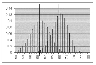
One question that may remain is, Why are the probabilities found from these two views not exactly the same? The answer lies in the fact that the binomial distribution is not symmetrical. The closer the actual proportion gets to 0 or to 1, the more the binomial distribution becomes skewed in the direction away from the 0 or 1 limit. This means that in most cases, the probabilities examined in the two ways given earlier will not be exactly equal. An example of a situation in which they would be equal could be given as the following: What is the probability that the true proportion of the population is 0.55 if a sample of eighty finds a proportion of 0.45? In this case, the two proportions are equidistant from the center of the probability distribution, which is 0.5. The proportion 0.55 of eighty is forty-four and 0.45 of eighty is thirty-six. Now if we use =BINOMDIST(36,80,0.55,1), we discover that the probability of finding thirty-six or fewer out of eighty when the probability is 0.45 is 0.046. If we use 1 -(=BINOMDIST(43,80,0.45,1)), we discover that the probability of finding forty-four or more out of eighty is 0.046. This happens because 0.45 and 0.55 are equidistant on opposite sides of 0.5, so their “skewnesses” are mirror images of one another.
The fact that the two different decision rules may not always produce the same probability should not be a source of great concern. In most cases, the probabilities will differ only slightly. Only infrequently would a different decision be reached from one view versus the other.

EXERCISES FOR SECTION 5.3
1. Use Equation 5.6 to determine the probability of any one outcome of the following:
a. n = 5, x = 2, p = 0.646
b. n = 11, x = 9, p = 0.42
c. n = 11, x = 7, p = 0.42
d. n = 120, x = 35, p = 0.5
e. n = 120, x = 60, p = 0.5
2. Use Equation 5.7 to determine the number of separate outcomes for the following:
a. n = 5, x = 2
b. n = 11, x = 9
c. n = 11, x = 7
d. n = 120, x = 35
e. n = 120, x = 60
3. Use Equation 5.8 to determine the binomial probability of the following:
a. n = 5, x = 2, p = 0.646
b. n = 11, x = 9, p = 0.42
c. n = 11, x = 7, p = 0.42
d. n = 120, x = 35, p = 0.5
e. n = 120, x = 60, p = 0.5
4. Use the =BINOMDIST() function to determine the binomial probability of the following and determine if they are the same as what is given in Exercise 3.
a. n = 5, x = 2, p = 0.646
b. n = 11, x = 9, p = 0.42
c. n = 11, x = 7, p = 0.42
d. n = 120, x = 35, p = 0.5
e. n = 120, x = 60, p = 0.5
5. Use the formulas in Equations 5.6, 5.7, and 5.8 to replicate Figure 5.15.
a. Add the comparable values as generated by the =BINOMDIST() function as column D.
b. Add the cumulative probabilities as column E by accumulating column C from x = 0.
c. Add the cumulative probabilities as column F by using =BINOMDIST() with 1 as the final argument.
d. Do columns C and D and columns E and F match?
6. A local health department counsels expectant mothers coming to a prenatal clinic on cigarette smoking only if they are smokers. History has shown that about 27 percent of expectant mothers are smokers when they first come to the clinic. Assume that the clinic will see eleven new expectant mothers today.
a. Use the formulas in Equations 5.6, 5.7, and 5.8 to determine binomial probabilities that the health department will see no women who smoke today, one woman who smokes, two women who smoke, and so on, up to eleven women who smoke.
b. Use =BINOMDIST() to determine the same values.
c. Accumulate the values found in (a) (preceding) from 0 to 11.
d. Use =BINOMDIST() to determine the cumulative probabilities.
e. Make sure that the two sets of probabilities are equal to each other.
7. A dentist sees about fifteen new patients per month (the rest of her patients are repeats). She knows that on average, over the past year, about half of her patients have needed at least one filling on their first visit.
a. What is the probability that she will see ten patients or more out of fifteen who need fillings?
b. What is the probability that she will see five or fewer patients who need fillings?
c. What is the probability that she will see between seven and ten new patients who need fillings?
8. An emergency room administrator wants to know the proportion of emergency room patients who spend more than one hour before being attended to. He knows that the time of arrival at the emergency room and the time of seeing the first medical staff member are both recorded. He draws a random sample of fifty records and discovers fourteen indicate that the person spent more than one hour in waiting.
a. What is the probability that the true proportion of persons spending more than one hour is 36 percent or more?
b. What is the probability that the true proportion of persons spending more than one hour is 20 percent or less?
c. What is the probability that the true proportion of persons spending more than one hour is from 24 to 32 percent?
5.4 THE POISSON DISTRIBUTION
The Poisson distribution, like the binomial distribution, is a discrete distribution. It takes on values for whole numbers only. But whereas the binomial distribution is concerned with the probability of two outcomes over a number of trials, the Poisson distribution is concerned with the number of observations that will occur in a small amount of time or over a region of space. We have been discussing the probability of seeing a certain number of emergencies out of a number of persons who arrive at an emergency room. The binomial distribution describes these probabilities. But if we consider the actual arrival at the emergency room of anyone, emergency or not, the Poisson distribution is more likely to describe these probabilities.
Arrivals at the Emergency Room: Application of the Poisson Distribution Consider again the emergency room that deals with twenty-nine people, on average, during an administrator’s eight-hour shift. The administrator can figure out that this is an average of just about 0.9 persons—or just less than one person—every fifteen minutes. She also knows that it takes about fifteen minutes to go through all the administrative paperwork—checking insurance coverage, inquiring about previous visits, and so on—entailed in getting a person into the system. She knows that she will have to be prepared to deal with about one person every fifteen minutes, but she also knows that on occasion several people arrive within the same fifteen-minute time interval, even when they arrive for different reasons. She would like to know, then, how often she will have to be prepared to deal with two people, or three or four, in any fifteen-minute interval. She can determine this with the Poisson distribution.
The =POISSON() Function in Excel Figure 5.20 shows the Poisson-predicted probabilities for the number of arrivals in any fifteen-minute period. The probabilities are calculated using the =POISSON() function, which takes three arguments. These are the number of arrivals (A2 in the formula line), the average number of arrivals during the period of time under consideration ($B$11 in the formula line, and generally termed l in the context of the Poisson distribution), and a zero to indicate that the actual probability is desired.
FIGURE 5.20 Poisson distribution of emergency room arrivals in fifteen-minuteintervals
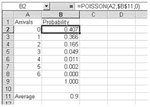
It is important to point out that the probabilities shown in Figure 5.20 are based on three assumptions:
• The arrival of an emergency in any fifteen-minute interval is independent of arrivals in any other fifteen-minute interval.
• The number of arrivals in the time interval is proportional to the size of the interval.
• The likelihood of more than one arrival in the time interval is very small.
If the administrator accepts these assumptions, she can see from Figure 5.20 that in only a small number of fifteen-minute intervals will she have to deal with more than two arrivals in the same fifteen-minute interval. The specific probability is calculated as follows: 0.063 × 32 = 2.01, or about two in any eight-hour shift. (Note: The 32 is four fifteen-minute intervals over eight hours and the 0.063 is the sum of cells B5 through B8 in Figure 5.20.) Moreover, she will have to deal with more than three arrivals in a fifteen-minute period in only about one fifteen-minute interval in any two eight-hour shifts (0.013 × 32 = 0.416). On this basis, she may be well justified in being prepared to deal with up to two arrivals in a fifteen-minute period but in letting the arrival of three or more persons be treated as an unlikely event that will be handled by the mobilization of extra resources.
Equations for the Poisson Distribution
In the section on the binomial distribution, we spent a good deal of time showing where the binomial distribution comes from. This was for two reasons:
• The binomial distribution is a relatively easy distribution to understand.
• The number of different combinations of any outcome (HHTHT, for example) is a general formula that applies to many different aspects of statistics.
The Poisson distribution, however, is more difficult to derive. So in the case of the Poisson distribution, we will look at the formula for the distribution directly. The formula for the Poisson distribution is shown in Equation 5.9.

Equation 5.9 says that the probability of any value x is equal to the quantity δ to the power of x times e to the power of -δ, divided by x! for 0 and integer values of x, but 0 for noninteger values of x. Like the binomial distribution, the Poisson distribution is defined only for 0 and integers. The term e-δ is the value of e (approximately 2.718) raised to the negative power of the mean number of arrivals in any given interval of time.
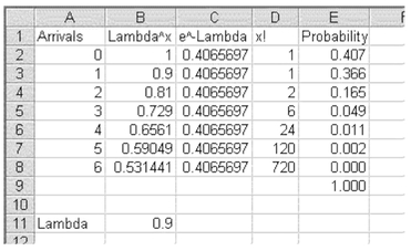
FIGURE 5.21 Calculated Poisson distribution of emergency room arrivals in fifteen-minute intervals
Calculating the Poisson Distribution with a Spreadsheet
Figure 5.21 shows the calculated values of the Poisson distribution for emergency room arrivals in fifteen-minute intervals. Column B gives the value of δx, where x represents zero to six arrivals. Column C is simply the value of e (2.718) raised to the power of -δ. Column D is the factorial value for each number of arrivals, zero to six. Column E uses the formula in Equation 5.9 to replicate the values in column B in Figure 5.20.
Figure 5.22 shows the Excel formulas for the calculations in Figure 5.21. The calculations in column C use the Excel =EXP() function, which raises the value of e to the power of the value in the parentheses. The calculations in column D use the =FACT() function, which provides the factorial of the number in parentheses. Both of these functions take only one argument. The formulas shown in Figure 5.22 are revealed in Excel by the selection of Tools Options from the menu bar and the checking of the Formula box on the View tab.
Poisson distributions apply not only to the distribution of occurrences in short periods of time but also to occurrences in regions. For example, suppose a hospital supply room is responsible for maintaining a supply of rubber gloves. The gloves come in boxes of one hundred, and quality control is advertised to be very good concerning these gloves. However, the hospital supply room manager has found that he gets reports of an average of about two gloves in every box of one hundred that are not usable for one reason or another. Given this information, what is the probability that in any given box of gloves, all will be usable? What is the probability that only one will not be usable, or that more than five will not be usable? This can also be found by using the Poisson distribution.
FIGURE 5.22 Calculated Poisson distribution of emergency room arrivals: Excel formulas
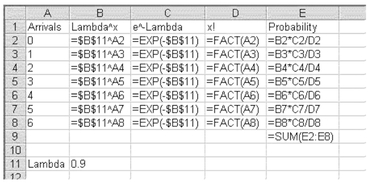
FIGURE 5.23 Poisson distribution for gloves that are not usable in a box of one hundred
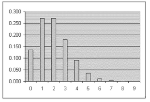
Figure 5.23 charts the distribution of probabilities for the number of gloves that will be unusable in a box of one hundred if the average number unusable in a box is two (e.g., for a spreadsheet model use =POISSON(x,2,0)). The supply room manager can expect about 14 percent of the boxes to have all good gloves (x=0); an equal number, about 27 percent, to have one or two unusable gloves (x=1 or x=2); and about 18 percent to have three unusable gloves (x=3). A very small percent of boxes will have as many as eight unusable gloves.

EXERCISES FOR SECTION 5.4
1. Replicate the Poisson distribution for persons arriving at the emergency room, as is shown in Figure 5.20, using
a. The =POISSON() function
b. The Poisson formula shown in Equation 5.9
2. Calculate the Poisson probabilities for finding unusable gloves in a box of one hundred if the average is two per box
a. Using the =POISSON() function
b. Using the Poisson formula shown in Equation 5.9
c. Replicate the chart in Figure 5.23.
5.5 THE NORMAL DISTRIBUTION
The last topic that will be taken up in this chapter is the normal distribution. Both the binomial distribution and the Poisson distribution describe discrete numerical variables. That is, they give the probability of a certain number of true emergencies among visitors to an emergency room. Discrete events are individually distinct and take on a finite or countable number of values.
Continuous Probability Distributions
The normal distribution, however, provides probabilities for continuous numerical variables. Height of adult males, for example, is a continuous variable. Body temperature is another continuous variable, as is pulse rate or blood pressure. The amount of time spent in a physician’s waiting room or with the physician is a continuous variable. All of these variables can be determined not by counting, which can be done with a discrete variable, but by measurement. In general, it is reasonable to say that a continuous numerical variable is the result of some measurement—say, with a watch, a ruler, or a scale.
Discrete distributions contain a finite or countable number of values. Continuous distributions contain an infinite or noncountable number of values.
The normal distribution is just one of a number of distributions that describe the properties of continuous numerical data. However, in terms of elementary statistical applications, it is by far the most important and is the only continuous distribution treated in any detail in this text. The chi-square distribution and the F distribution, both continuous distributions, will be discussed, but only as these apply to hypothesis testing.
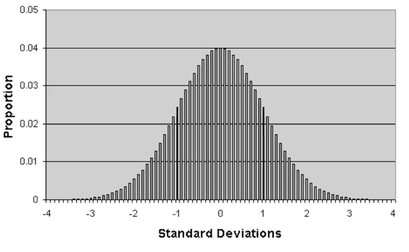
FIGURE 5.24 A normal distribution
An Introduction to the Normal Distribution
To briefly introduce the normal distribution, consider the chart shown in Figure 5.24. This chart represents the normal distribution. The normal distribution is discussed in detail in chapter six, but several points about it are noteworthy here. First, the normal distribution has often been called a bell-shaped curve because it looks like the cross-section of a bell. Second, because the normal distribution looks like a bell, both sides of the distribution have exactly equal probabilities. In other words, the normal distribution is symmetrical. For example, if the probability of being at the point -1 on the horizontal scale is 0.024, then the probability of being at 1 on the horizontal scale is also 0.024. Moreover, the probability of being between -3 and 0 is exactly the same as being between 0 and 3.
Standard Deviation and the Normal Distribution
In Figure 5.24, the horizontal axis is given as standard deviations. The meaning of the term “standard deviation” is discussed in detail in chapter six. So, for now we will use the term in the context of the normal distribution. It is sufficient to say that in any normal distribution, approximately 68 percent of all observations will be within ±1 standard deviation of the center of the distribution. Let’s assume we have a normally distributed data set of average height of adult males. Consequently, then it can be expected that in a large sample of adult males, 68 percent will have heights no less than one standard deviation below the average and no more than one standard deviation above the average. Furthermore, if the average height of adult males is normally distributed, 95 percent of all adult males will have heights between ±2 standard deviations of the average. Following this logic, 99 percent will have heights between ±3 standard deviations of the average.
Three Common Characteristics of the Normal Distribution: 68 Percent, 95 Percent, and 99 Percent
The average height of adult males in the United States is about sixty-nine inches. Let us say that virtually all adult U.S. males are at least sixty inches tall and no more than seventy-eight inches tall. Of course, there are some U.S. adult males—professional basketball players, for example—who are notably taller than seventy-eight inches. In fact, this is also a characteristic of normal distributions. Normal distributions have no upper or lower limits. If the range of adult human height is sixty to seventy-eight inches and if height is normally distributed, then we could say that the standard deviation of height is about three inches (78 - 60 = 18, 18/6 = 3). Consequently, we could say that 68 percent of all U.S. males are between sixty-six and seventy-two inches tall (e.g., 69 ± 1*3 = 66 and 72). Furthermore, we could say that 95 percent of all adult males are between sixty-three and seventy-five inches tall (e.g., 69 ± 2*3 = 63 and 75). Finally, 99 percent are between sixty and seventy-eight inches tall (e.g., 69 ± 3*3 = 60 and 78).
The following can be said about a normal distribution:
• Approximately 68 percent of the values lie between ± 1 standard deviation from the mean.
• Approximately 95 percent of the values lie between ± 2 standard deviations from the mean.
• Approximately 99 percent of the values lie between ± 3 standard deviations from the mean.
The use of height to discuss the normal distribution is not accidental. Height is a measure. On the measurement scale of height, a person may be at any point. He does not need to be exactly sixty-nine inches tall (although we might measure him as such). The normal probability distribution is a distribution of measurement. This is in contrast to both the binomial probability distribution and the Poisson probability distribution, which are both distributions of events or counts. Because the normal distribution is a distribution of measures, it is a continuous numerical probability distribution. More is said about the consequence of this fact in chapter six.
KEY TERMS
=BINOMDIST()
=EXP()
=FACT()
=POISSON()
contingency table
empirical probability
event
independence
joint probability
marginal probability
mutually exclusive
a priori
bell-shaped curve
binomial distribution
conditional probability
normal distribution
outcome
Poisson distribution
probability
sample space
standard deviation
stochastic process
..................Content has been hidden....................
You can't read the all page of ebook, please click here login for view all page.
