

436 Stochastic volatility modeling
20%
25%
30%
35%
40%
45%
50%
50% 70% 90% 110% 130% 150%
1 month
6 months
1 year
2 years
5 years
15%
20%
25%
30%
50% 70% 90% 110% 130% 150%
1 month
6 months
1 year
2 years
5 years
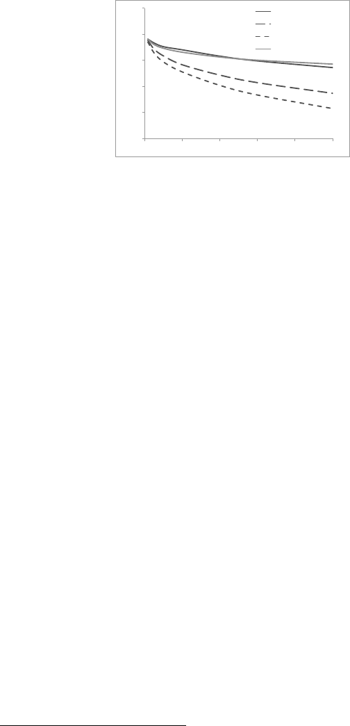
Figure 11.2
: Left: component’s smile with parameters of Table 11.3. Right: basket
smile with ρ
SS
= 60%, χ
Sσ
= 0 and χ
σσ
= 0.
10%
15%
20%
25%
30%
35%
40%
50% 70% 90% 110% 130% 150%
1 month
6 months
1 year
2 years
5 years
10%
15%
20%
25%
30%
35%
40%
50% 70% 90% 110% 130% 150%
1 month
6 months
1 year
2 years
5 years
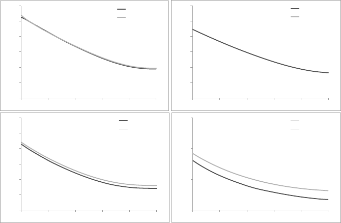
Figure 11.3
: Basket smile with:
ρ
SS
= 60%, χ
σσ
= 80%
. Left:
χ
Sσ
= 80%
. Right:
χ
Sσ
= 115%.
Comparing with the left-hand graph in Figure 11.2 it is apparent that the basket
ATMF skew with (
χ
Sσ
= 115%, χ
σσ
= 80%
) is now steeper than the component’s
ATMF skew.
How accurate are formulas for (11.24),(11.30) for S
B
T
, ˆσ
B
T
?
Basket ATMF skew
Figure (11.4) shows the 95/105 ATMF basket skew (
ˆσ
B
K=0.95S
0
,T
− ˆσ
B
K=1.05S
0
,T
),
either calculated in a Monte Carlo simulation, or evaluated using (11.24), with
S
T
given either by the actual component’s ATMF skew, or given by (11.27), for two
dierent values of
χ
Sσ
. The left-hand graph conrms that expression (11.24) is very
accurate. The small overestimation of
S
B
T
in the right-hand graph is due to the slight
overestimation of the component’s skew in (11.27), evidenced in Figure 8.3, page
331.
Figure (11.5) provides another conrmation that the basket ATMF skew is con-
trolled by
χ
Sσ
. Here we have varied
χ
σσ
while keeping
ρ
SS
= 60%
and
χ
Sσ
= 80%
xed. The ATMF skew hardly changes when
χ
σσ
is varied. For the three values

Multi-asset stochastic volatility 437
0%
1%
2%
3%
4%
5%
6%
7%
0 1 2 3 4 5
Actual χSσ = 115%
Approx χSσ = 115%
Actual χSσ = 80%
Approx χSσ = 80%
0%
1%
2%
3%
4%
5%
6%
7%
0 1 2 3 4 5
Actual χSσ = 115%
Approx χSσ = 115%
Actual χSσ = 80%
Approx χSσ = 80%
Figure 11.4
: Left: basket 95/105 skew in volatility points (Actual) compared to
formula (11.24) (Approx) where the actual component’s 95/105 skew has been used.
Right: basket 95/105 skew (Actual) compared to formula (11.28) (Approx). Maturities
are in years. The two values of
χ
Sσ
= 80%, 115%
have been used. All other
parameters are kept constant, including χ
σσ
= 80%.
10%
15%
20%
25%
30%
35%
40%
60% 80% 100% 120% 140%
χσσ = 40%
χσσ = 80%
χσσ = 95%
Figure 11.5
: One-year basket smiles for dierent values of
χ
σσ
. All other parameters
are kept constant: ρ
SS
= 60% and χ
Sσ
= 80%.
of
χ
σσ
used:
40%, 80%, 95%
, the 95/105 one-year skew values are respectively:
2.01%, 2.05%, 2.06%.
Using identical and at term structures of VS volatilities for the basket compo-
nents, as well as identical sets of parameters, leads to the particularly simple formulas
(11.24) and (11.28) but the derivation of
S
B
T
in the general case presents no particular
diculty. One only needs to express
µ
B
(t, u)
as a function of the component’s
spot/volatility covariance functions
µ(t, u, ξ)
, which are given by expression (8.50)
in the two-factor model.
Basket VS volatility
ˆσ
B
T
, either evaluated in a Monte Carlo simulation or given by (11.30), is graphed in
Figure 11.6 for dierent values of
χ
Sσ
. In expression (11.30), with the approximation
438 Stochastic volatility modeling
20%
21%
22%
23%
24%
25%
0 1 2 3 4 5
Actual χSσ = 115%
Actual χSσ = 80%
Actual χSσ = 40%
Approx
Figure 11.6
:
ˆσ
B
T
, either evaluated in a Monte Carlo simulation of the two-factor
model, for three values of
χ
Sσ
: 40%, 80%, 115%
, or given by expression (11.30).
Maturities are in years. The component’s parameters are listed in Table 11.3 and
ρ
SS
= 60%, χ
σσ
= 80%.
of frozen weights, only spot/spot (
ρ
SS
) and volatility/volatility (
χ
σσ
) correlations
appear.
Figure 11.6 makes it clear that this assumption is not adequate:
ˆσ
B
T
does depend
on cross spot/volatility correlations.
11.3.3 Mimicking the local volatility model
Can our two-factor stochastic volatility model mimic a multi-asset local volatility
model? In the local volatility model,
ρ
cross
(S, bσ
T
) = −ρ
SS
and
ρ
cross
(bσ
T
, bσ
T
0
) =
ρ
SS
. We have:
ρ
diag
(S, bσ
T
) = −1
and
ρ
diag
(bσ
T
, bσ
T
0
) = 1
.
7
Thus, in the local
volatility model:
ρ
cross
(S, bσ
T
) = ρ
SS
ρ
diag
(S, bσ
T
)
ρ
cross
(bσ
T
, bσ
T
0
) = ρ
SS
ρ
diag
(bσ
T
, bσ
T
0
)
Thus, with regard to spot/volatility and volatility/volatility correlations, the
local volatility model can be viewed as a particular breed of multi-asset stochastic
volatility with χ
Sσ
, χ
σσ
given by:
χ
Sσ
= ρ
SS
(11.31a)
χ
σσ
= ρ
SS
(11.31b)
With this choice of cross-parametrization the values of
ζ
in (11.17) are both equal
to 1, thus positivity conditions are satised.
7
We use here
ρ
diag
(S, bσ
T
) = −1
as we are considering the typical case of negatively sloping equity
smiles. We could equivalently have written ρ
diag
(S, bσ
T
) = 1.
Multi-asset stochastic volatility 439
It is easy to check that in case spot/spot correlations are not all equal, the
correlation structure of the multi-asset local volatility model is still given by (11.31)
with
ρ
SS
,
χ
Sσ
,
χ
σσ
adorned with
ij
superscripts, as
ρ
cross
(S
i
, bσ
j
T
) = −ρ
ij
SS
and
ρ
cross
(bσ
i
T
, bσ
j
T
0
) = ρ
ij
SS
.
We now test this mapping with the same parameter values used in Section 11.3.2;
ρ
SS
= 60%
. We use two-factor-model parameters in Table 11.3 to generate a vanilla
smile. Using this as the component’s vanilla smile, we calibrate the component’s
local volatility function and price the basket smile using ρ
SS
= 60%.
We then compare the resulting basket smile with that produced by our multi-
asset two-factor model with
χ
σσ
= χ
Sσ
= ρ
SS
= 60%
. Results appear in Figure
11.7.
It is apparent that the mapping (11.31) is accurate for short maturities; for longer
maturities implied volatilities in the stochastic volatility model are lower than in
the local volatility model. This is not surprising: because volatilities – especially
forward volatilities – are more volatile in the stochastic volatility model than in the
local volatility model: the level of “eective” spot/spot correlation is lower than
ρ
SS
.
This aects all multi-asset products, including the correlation swap which we now
study.
10%
15%
20%
25%
30%
35%
40%
70% 80% 90% 100% 110% 120%
1 month
Stoch vol
Local vol
10%
15%
20%
25%
30%
35%
40%
70% 80% 90% 100% 110% 120%
3 months
Stoch vol
Local vol
10%
15%
20%
25%
30%
35%
40%
50% 70% 90% 110% 130% 150%
1 year
Stoch vol
Local vol
15%
20%
25%
30%
50% 70% 90% 110% 130% 150%
5 years
Stoch vol
Local vol
Figure 11.7
: Comparison of basket smiles in local volatility and stochastic volatility
models, for several maturities. The mapping of local to stochastic volatility is obtained
with
χ
σσ
= χ
Sσ
= ρ
SS
= 60%
. The basket consists of
n = 10
components, with
identical smiles given by parameters in Table 11.3.

440 Stochastic volatility modeling
11.4 The correlation swap
Consider a basket of stocks or indexes. A correlation swap of maturity
T
pays at
T
the average pairwise realized correlation of the basket components minus a xed
strike bρ
1
n(n −1)
X
i6=j
ρ
ij
− bρ (11.32)
where
bρ
is set so that the swap’s initial value vanishes. Correlation
ρ
ij
of
S
i
,
S
j
is
dened with the standard realized correlation estimator, using daily log-returns:
ρ
ij
=
Σr
i
k
r
j
k
q
Σ r
i
k
2
q
Σ r
j
k
2
(11.33)
where
r
i
k
= ln(S
i
k
/S
i
k−1
)
and the sums runs from
k = 1
to
k = N
, where
N
is the
number of returns used for estimating covariances and variances in (11.33).
n
is the number of securities: 2 or 3 when the components are indexes and up to
50 for a correlation swap on the constituents of the Euro Stoxx 50 index. We have
used in (11.32) the typical equal weighting.
Strike
bρ
is also called the implied correlation of the swap. Indeed, in a constant
volatility model, for daily returns, with all spot/spot correlations
ρ
SS
equal and a
large number of returns – thus a long maturity – bρ = ρ
SS
.
For shorter maturities, (11.33) is biased. Let us make the assumption of centered
log-returns:
r
i
k
= σ
i
√
∆tZ
i
k
, where
σ
i
is the (constant) volatility of asset
i
,
∆t
the
interval between two spot observations – here one day, and the
Z
i
k
are iid standard
normal random variables.
The bias and standard deviation of the correlation estimator are derived in
Appendix A, at lowest order in
1
N
:
E[ρ
ij
] = ρ
SS
1 −
1 −ρ
2
SS
2N
(11.34)
Stdev (ρ
ij
) =
1
√
N
1 −ρ
2
SS
(11.35)
where
N
is the number of returns in the historical sample. Typically the bias in
E[ρ
ij
] is about one point of correlation for ρ
SS
= 60% and T = 1 month.
Correlation swaps were introduced as a means of trading correlation and making
implied correlation an observable parameter.
As a measure of correlation, however, averaging pairwise correlations results in
a poorly dened estimator.
One would expect of an adequately dened estimator that its standard deviation
vanishes either in the limit of a large sample size (
N → ∞
) or as the number of
..................Content has been hidden....................
You can't read the all page of ebook, please click here login for view all page.