Eigenvalues and Eigenvectors
It was shown in Chapter 6 that provided the eigenvalues and eigenvectors of a system can be found, it is possible to transform the coordinates of the system from local or global coordinates to coordinates consisting of normal or ‘principal’ modes.
Depending on the damping, the eigenvalues and eigenvectors of a system can be real or complex, as discussed in Chapter 6. However, real eigenvalues and eigenvectors, derived from the undamped equations of motion, can be used in most practical cases, and will be assumed here, unless stated otherwise.
In Example 6.3, we used a very basic ‘hand’ method to demonstrate the derivation of the eigenvalues and eigenvectors of a simple 2-DOF system; solving the characteristic equation for its roots, and substituting these back into the equations to obtain the eigenvectors. In this chapter, we look at methods that can be used with larger systems.
7.1 The eigenvalue problem in standard form
In Chapter 6, it was shown that the undamped, homogeneous equations of a multi-DOF system can be written as:
or concisely,
wheer
[M] is the (n × n), symmetric, mass matrix, [K] the (n × n), symmetric, stiffness matrix, ω any one of the n natural frequencies and {![]() } the corresponding (n × 1) eigenvector.
} the corresponding (n × 1) eigenvector.
Putting λ = ω2, Eq. (7.2) can be written as:
where λ is any one of the n eigenvalues.
In order to take advantage of standard mathematical methods for extracting eigenvalues and eigenvectors, Eq. (7.3) must usually be converted to the ‘standard form’ of the problem. This is the purely mathematical relationship, known as the algebraic eigenvalue problem:
where the square dynamic matrix, [A], is, as yet, undefined.
Equation (7.4) is often written as:
where the unit matrix [I] is introduced, since a column vector cannot be subtracted from a square matrix.
In Eqs (7.4) and (7.5), although λ is shown as a single scalar number, it can take n different values, where n is the number of degrees of freedom. Similarly, n corresponding eigenvectors, {![]() }, can be found.
}, can be found.
There are now two ways in which Eq. (7.3) can be expressed in the standard form of Eq. (7.5):
(1) The first method is to pre-multiply Eq. (7.2) through by [M]−1, giving:
Since [M]−1 [M] = [I], the unit matrix, this is now seen to be in the standard form of Eq. (7.5):
where [A] = [M]-1[K]; and λ = ω2.
(2) The second method is to pre-multiply Eq. (7.2) through by [K]−1, giving:
Since [K]−1 [K] = [I], this is also seen to be in the standard form of Eq. (7.5):
where ![]()
The matrices [A] and [![]() ] are not the same, but both can be referred to as the dynamic matrix. In general, these matrices are not symmetric, even though both [M] and [K] are. The eigenvectors, {
] are not the same, but both can be referred to as the dynamic matrix. In general, these matrices are not symmetric, even though both [M] and [K] are. The eigenvectors, {![]() }, given by the two methods are identical, but it can be seen that the eigenvalues produced by the two methods are not the same. In the first case, λ = ω2, and in the second case,
}, given by the two methods are identical, but it can be seen that the eigenvalues produced by the two methods are not the same. In the first case, λ = ω2, and in the second case, ![]() .
.
Both of the above ways of defining the dynamic matrix, are in common use. It should be noted that the first method uses the stiffness matrix, [K], and the second method uses the flexibility matrix, [K]−1.
There are many methods for extracting eigenvalues and eigenvectors from the dynamic matrix, and some of these are discussed in Section 7.2.
7.1.1 The Modal Matrix
When matrix transformation methods are used, it is often convenient to form the eigenvectors into a single matrix known as the modal matrix. Then Eq. (7.3),
can be written as:
where [Φ] is the modal matrix formed by writing the eigenvectors as columns:
and [Λ] is a diagonal matrix of the eigenvalues:
Similarly, when the equation is in the form of a dynamic matrix, such as Eq. (7.5),
it can be written as:
where [Φ] and [Λ] are defined by Eqs (7.11) and (7.12), respectively.
In Eq. (7.3), although it is possible to find n eigenvalues and n corresponding eigenvectors, they do not necessarily all have to be extracted. This may be justifiable on physical grounds; for example, we may not be interested in the response of the system above a maximum frequency component in the applied forcing. Therefore, although the matrices [M] and [K] in the foregoing discussion will always be of size n × n, as will the dynamic matrix [A] or [![]() ], the modal matrix, [Φ], may be a rectangular matrix of size n × m (i.e. n rows and m columns), where m ≤ n. The diagonal matrix of eigenvalues, [Λ], will then be of size m × m. It should be pointed out, however, that some methods for extracting eigenvalues and eigenvectors require all n to be found.
], the modal matrix, [Φ], may be a rectangular matrix of size n × m (i.e. n rows and m columns), where m ≤ n. The diagonal matrix of eigenvalues, [Λ], will then be of size m × m. It should be pointed out, however, that some methods for extracting eigenvalues and eigenvectors require all n to be found.
7.2 Some basic methods for calculating real eigenvalues and eigenvectors
Only a brief introduction to this quite complicated subject can be given. The following basic methods are described in this section:
(a) Eigenvalue (only) extraction from the roots of the characteristic equation. The eigenvectors can then be found by substituting the eigenvalues back into the equations, and extracted using one of several methods, of which Gaussian elimination is used as an example below.
(b) Matrix iteration, giving both the eigenvalues and the eigenvectors.
(c) Jacobi diagonalization. The Jacobi method requires a symmetric dynamic matrix as input, and since [A] and [![]() ] are not naturally symmetric, this must first be arranged. If both the mass and the stiffness matrices are fully populated, Choleski factorization is used to ensure that the dynamic matrix is, in fact, symmetric. If, as is often the case, either the mass matrix or the stiffness matrix is diagonal, a much simpler method can be used.
] are not naturally symmetric, this must first be arranged. If both the mass and the stiffness matrices are fully populated, Choleski factorization is used to ensure that the dynamic matrix is, in fact, symmetric. If, as is often the case, either the mass matrix or the stiffness matrix is diagonal, a much simpler method can be used.
7.2.1 Eigenvalues from the Roots of the Characteristic Equation and Eigenvectors by Gaussian Elimination
Finding the eigenvalues from the roots of the characteristic equation has already been demonstrated for a 2 × 2 set of equations in Example 6.3. The following example further illustrates the method, and goes on to find the eigenvectors by Gaussian elimination.
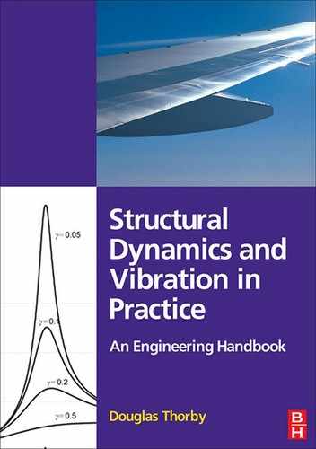
(a) Find the eigenvalues, and hence the natural frequencies, of the undamped 3-DOF system shown in Fig. 7.1, by solving the characteristic equation for its roots.
(b) Using the eigenvalues, find the eigenvectors by Gaussian elimination.
The numerical values of the masses m1, m2 and m3, and the stiffnesses, k1, k2 and k3, are as follows:
| m1 = 2 kg; | m2 = 1 kg; | m3 = 2 kg; |
| k1 = 1000 N/m; | k2 = 0000 N/m; | k3 = 1000 N/m; |
Part (a):
The stiffness matrix for the springs of this system was derived in Example 1.4. Using the method described in Section 6.1.2, the equations for the undamped unforced system are as follows:
Substituting {z} = {![]() }eiωt in the usual way, and inserting the numerical values gives
}eiωt in the usual way, and inserting the numerical values gives
Substituting ω2 = λ and introducing the scaling ![]() to simplify the matrices:
to simplify the matrices:
The determinant D of Eq. (C) is now equated to 0:
Using the standard rule for evaluating a determinant:
which when simplified gives
Using a standard roots solution program, the scaled roots, ![]() , as calculated, are:
, as calculated, are:
However, since the roots, ![]() , were defined as
, were defined as ![]() = 10−3λi, the eigenvalues of the physical problem, λi, are
= 10−3λi, the eigenvalues of the physical problem, λi, are
The natural frequencies, ωi, in rad/s are
From Eq. (C):
The scaled roots ![]() are now substituted, one at a time, into Eq. (G), and Gaussian elimination is used to find the corresponding eigenvectors. Substituting the first root,
are now substituted, one at a time, into Eq. (G), and Gaussian elimination is used to find the corresponding eigenvectors. Substituting the first root, ![]() = 0.1401, into Eq. (G) gives
= 0.1401, into Eq. (G) gives
The vector has the subscript (1) to indicate that it is the eigenvector corresponding to the first eigenvalue.
Gaussian elimination is a standard method for solving any set of linear equations. The general idea is to eliminate the terms in the matrix below the leading diagonal, then the values of ![]() can be found by back-substitution.
can be found by back-substitution.
In this case the term −2 in the first column can be removed by multiplying the first row by (−2/2.7198) = −0.7353 and subtracting it from the second row, giving
Without going further, from Eq. (I) we have the ratios:
If ![]() is now arbitrarily assigned the value 1, then the first eigenvector is
is now arbitrarily assigned the value 1, then the first eigenvector is
The second eigenvector can be found in precisely the same way, by substituting the second scaled root, ![]() = 0.9017, into Eq. (G), and repeating the process of eliminating terms below the diagonal and so on. The whole process is then repeated for the third eigenvector.
= 0.9017, into Eq. (G), and repeating the process of eliminating terms below the diagonal and so on. The whole process is then repeated for the third eigenvector.
7.2.2 Matrix Iteration
This method extracts both eigenvalues and eigenvectors from the dynamic matrix. Its use is illustrated by the following example, where the flexibility matrix [K]−1 rather than the stiffness matrix [K] is used. Since the matrix iteration method always finds the mode with the largest eigenvalue first, it can be seen from Eq. (7.9) that this will correspond to the lowest natural frequency, and this is usually desirable.
(a) Basing the calculation on the flexibility matrix, use the matrix iteration method to find the eigenvalue and eigenvector of the lowest frequency mode of the 3-DOF system of Example 7.1.
Part (a):
Although we intend to base the calculation on the flexibility matrix, [K]−1, suppose for a moment that the homogeneous equations of motion, in terms of the stiffness matrix, [K], are
Substituting {z} = {![]() }eiωt in the usual way:
}eiωt in the usual way:
leads to a standard form
where
The flexibility matrix [K]−1 for the same system was derived in Example 1.4 as:
Inserting the numerical values, the matrices [M], [K]−1 and [![]() ] become
] become
Equation (D), to be solved by matrix iteration, is then,
where
To find the first eigenvector {![]() }1 and first scaled eigenvalue,
}1 and first scaled eigenvalue, ![]() , a trial vector, {
, a trial vector, {![]() }, say,
}, say,
is inserted on the left side of Eq. (F). The equation is then evaluated with this assumption, normalizing the resulting vector by dividing by the largest element:
The process is repeated, using the normalized column on the right in place of the trial vector on the left. After four such repeats, we have
The final vector on the right is now seen to agree with the first eigenvector from Example 7.1 by the Gaussian elimination method, to four significant figures. The root ![]() gives ω = 11.83 rad/s agreeing with the result of Example 7.1.
gives ω = 11.83 rad/s agreeing with the result of Example 7.1.
To find the second eigenvalue and eigenvector, the first eigenvector, already found, must be completely removed from the dynamic matrix [![]() ]. This can be achieved by using the orthogonality relationship, Eq. (6.54):
]. This can be achieved by using the orthogonality relationship, Eq. (6.54):
At some point in the iteration procedure, the impure vector {![]() } must consist of a linear combination of the three pure eigenvectors being sought
} must consist of a linear combination of the three pure eigenvectors being sought
where C1, C2 and C3 are constants. Pre-multiplying Eq. (K) by ![]() [M]:
[M]:
Now due to the orthogonality relationship for eigenvectors, Eq. (J), the last two terms in Eq. (L) must be zero, and
To produce a vector {![]() } free from {
} free from {![]() }1 we can now set C1 = 0, and since clearly
}1 we can now set C1 = 0, and since clearly ![]() , it must be true that
, it must be true that
or written out, using the notation:
from which
where
and
The known values of s1 and s2 can now be incorporated into a sweeping matrix, [S], where:
This is incorporated into the original iteration equation, Eq. (D), as follows:
and Eq. (F) becomes
or
This is then solved for the second eigenvector and second eigenvalue, in precisely the same way as before, using an estimated vector to start the process.
7.2.3 Jacobi Diagonalization
So far we have considered two forms of the eigenvalue problem: (1) From Eq. (7.7):
where
(2) From Eq. (7.9):
where
Unfortunately, both [A] and [![]() ] are non-symmetric matrices, and cannot be used directly in the Jacobi diagonalization, which requires the dynamic matrix to be symmetric. It can always be made symmetric, however, by applying a suitable transformation to the eigenvectors:
] are non-symmetric matrices, and cannot be used directly in the Jacobi diagonalization, which requires the dynamic matrix to be symmetric. It can always be made symmetric, however, by applying a suitable transformation to the eigenvectors:
where [U] is a square matrix, as yet undefined, equal in size to both [M] and [K], [U]−1 its inverse and {![]() } the transformed eigenvector.
} the transformed eigenvector.
To define the matrix [U], we return to Eq. (7.2):
and substitute Eq. (7.14) into it:
Equation (7.15) is now pre-multiplied by the transpose of [U]−1, i.e. ![]() , which can be written [U]−T:
, which can be written [U]−T:
We now consider two cases, which also define the matrix [U]:
We let [M]=[U]T[U], and substitute it into Eq. (7.16):
But since both [U]−T[U]T and [U][U]−1 are equal to [I], the unit matrix, Eq. (7.17) simplifies to
or
where λ = ω2 and
Let [K] = [U]T[U] and substitute this into Eq. (7.16):
which simplifies to
where in this case ![]() and
and
Equations (7.19) and (7.22) are both now in the standard form required, and the new dynamic matrix, whether it is [B], given by Eq. (7.20), or [![]() ], given by Eq. (7.23), depending upon which of the above methods is used, will be symmetric, as required for the Jacobi method of solution.
], given by Eq. (7.23), depending upon which of the above methods is used, will be symmetric, as required for the Jacobi method of solution.
The Jacobi method can now be used to find the eigenvalues and eigenvectors of either Eq. (7.19) or Eq. (7.22). To demonstrate the method we can represent either case by:
However, if [B] represents [B], then λ = ω2, but if [B] represents [![]() ], then λ = 1/ω2.
], then λ = 1/ω2.
For the Jacobi method, Eq. (7.24) is written in terms of the desired modal matrix, [Ψ], i.e. in the form of Eq. (7.13):
where
and [Λ] is the desired diagonal matrix of the eigenvalues, λi, these being equal to either ω2i or 1/ω2i, depending on whether the dynamic matrix was formed by using the method of Case 1 or Case 2 above.
The Jacobi method relies on the fact that, provided [B] is a symmetric, real matrix, then,
where [Ψ] and [Λ] are defined above.
If we apply a series of transformations [T1], [T2], [T3], etc., to [B] in the following way:
and so on, then provided the transformations are such that the off-diagonal terms in [B] are removed or reduced with each application, then [B] will eventually be transformed into [Λ], and the matrix of eigenvectors, [Ψ], will be given by the product of all the transformation matrices required to achieve this, i.e.,
Now a 2 × 2 symmetric matrix, say,  , can be transformed into diagonal form, in one operation, by a transformation matrix:
that is
It can be shown, by equating the terms in Eq. (7.31), that the value of θ required to achieve this is given by:
If it is desired to diagonalize a larger matrix, say the following 4 × 4 symmetric matrix,
it must be carried out in stages. The terms in [B](1) corresponding to b12 and b21, i.e. b(1)12 and b(1)21, where the superscript(1) indicates that these elements belong to [B](1), can be made zero by the transformation:
where
and θ1 is given by
Similarly, the terms b(2)24 and b(2)42 in [B](2) can be made zero by applying:
where
and
It may then be found that elements b(1)12 and b(1)21 in [B](2) have become non-zero, but their absolute values will be smaller than those of their original values, b12 and b21. Further sweeps may be necessary to reduce them, and all other off-diagonal terms, to some acceptably small tolerance.
This procedure is illustrated numerically in Example 7.3.
It must be remembered that the dynamic matrix was made diagonal by a coordinate change, Eq. (7.14),
and, of course, if the Jacobi method is used on the matrices [B] or [![]() ], the eigenvectors found will be the {
], the eigenvectors found will be the {![]() }, not the {
}, not the {![]() }. To obtain the eigenvectors relevant to the physical problem, {
}. To obtain the eigenvectors relevant to the physical problem, {![]() }, they must be transformed back, using the relationship {
}, they must be transformed back, using the relationship {![]() } = [U]−1{
} = [U]−1{![]() }.
}.
Although we have defined the matrix [U] as being given by either [M] = [U]T [U] or by [K] = [U]T[U], we have not yet discussed how it is evaluated. In general, if the matrices [M] and [K] are both non-diagonal, Choleski decomposition, described later in Section 7.3, will be required to find the matrix [U], and hence [U]T, [U]−1 and, [U]−T. However, if either [M] or [K] is diagonal, [U], [U]−1, etc. are of particularly simple form, and can be derived very easily. This is illustrated by the following example.
Use Jacobi diagonalization to find the eigenvalues and eigenvectors of the 3-DOF system used in Examples 7.1 and 7.2.
The equations of motion of the system can be written as:
where λ is an eigenvalue and {![]() } is an eigenvector. In numerical form, for this example:
} is an eigenvector. In numerical form, for this example:
Since the mass matrix is diagonal in this case, decomposing it into [M] = [U]T[U] is very easy since:
The inverse of [U], [U]−1 is found by simply inverting the individual terms:
From Eq. (7.19), the eigenvalue problem to be solved is
where from Eq. (7.20):
and λ = ω2.
A more convenient form of Eq. (G), using the modal matrix, [Ψ], is
where
and
Evaluating [B] from Eq. (H)
The end result of the Jacobi diagonalization that we are aiming for is, from Eq. (7.27),
So if we can find a series of transformations that eventually change [B] into [Λ], the product of these transformations must be the modal matrix, [Ψ]. The first transformation, aimed at reducing the b12 and b21 terms to zero, is
where
giving θ1 = 0.5416.
This has reduced the b(1)12 and b(1)21 terms to zero, as expected. We next reduce the b(1)23 and b(1)32 terms to zero by the transformation:
where
and
Applying Eq. (S): [B](2) = [T2]T[B](1)[T2], gives
This has reduced the b(1)23 and b(1)32 terms to zero, but the previously zero b(1)12 and b(1)21 terms have changed to 0.06291.
Three more transformations were applied, in the same way, with results as follows: Third transformation, θ3 = −0.6145:
Fourth transformation, θ4 = −0.0168:
Fifth transformation, θ5 = 0.0095:
This could be continued for one or two more transformations, to further reduce the off-diagonal terms, but it can already be seen that [B](5) has practically converged to a diagonal matrix of the eigenvalues. From Example 7.1, representing the same system, these were, in ascending order:
It will be seen that they appear in [B](5) in the different order: λ2, λ3, λ1.
The matrix of eigenvectors, [Ψ], is now given by Eq. (7.29). These are the eigenvectors of matrix [B], not those of the system, since it will be remembered that the latter were transformed by [U]−1 in order to make [B] symmetric. Since there were five transformations, [T1] through [T5], in this case, the eigenvectors [Ψ] are given by:
The final matrix product above, in the order in which it emerged from the diagonalization, is the modal matrix:
To find the eigenvectors, {![]() }, of the physical system, we must use Eq. (7.14):
}, of the physical system, we must use Eq. (7.14):
All the vectors can be transformed together by writing Eq. (7.14) as:
where [Φ] is the modal matrix of eigenvectors {![]() } and [Ψ] the modal matrix of eigenvectors {
} and [Ψ] the modal matrix of eigenvectors {![]() }. From Eq. (Y):
}. From Eq. (Y):
These are, finally, the eigenvectors of the system, {![]() }i, in the same order as the eigenvalues, i.e. {
}i, in the same order as the eigenvalues, i.e. {![]() }2, {
}2, {![]() }3, {
}3, {![]() }1. These would normally be rearranged into the order of ascending frequency.
}1. These would normally be rearranged into the order of ascending frequency.
As a check, we would expect the product [Φ]T[M][Φ] to equal the unit matrix, [I], and this is the case, to within four significant figures, showing that the eigenvectors emerge in orthonormal form, without needing to be scaled.
Another check is that the product [Φ]T [K] [Φ] should be a diagonal matrix of the eigenvalues, which is also the case to within four significant figures.
It should be noted that the presentation of the numerical results above, to about four significant figures, does not reflect the accuracy actually used in the computation.
7.3 Choleski factorization
In Example 7.3, advantage was taken of the fact that the mass matrix, [M], was diagonal, which enabled the transformation matrix [U]to be found very easily. It was then easy to form the dynamic matrix [B] in symmetric form, by Eq. (7.20), as:
This does not work if the matrices [M] and [K] are both non-diagonal, and in this, more general, case, Choleski factorization has to be used to find [U].
We saw in Section 7.2.3 that
(1) If the mass matrix [M] can be decomposed into [M]=[U]T[U], then the transformation [U]−T[M][U]−1 makes the mass matrix into a unit matrix and the transformation [U]−T[K][U]−1 makes the stiffness matrix symmetric.
(2) If the stiffness matrix [K] can be decomposed into [K]=[U]T[U], then the opposite happens, the transformation [U]−T[K][U]−1 produces a unit matrix, and [U]−T[M][U]−1 is a symmetric mass matrix.
Either way, the dynamic matrix becomes symmetric, as required by many eigenvalue/eigenvector extraction programs.
In the Choleski factorization, [U] is written as an upper triangular matrix of the form:
and its transpose [U]T is
This means that, depending on whether [U] is derived from [M]=[U]T[U] or from [K]=[U]T[U], the products [U]−T[K][U]−1 and [U]−T[M][U]−1 will either be equal to the unit matrix, [I], or be symmetric, and in either case a symmetric dynamic matrix will result.
It can now be seen why the matrix [U] is so named; it is because it is an upper triangular matrix. It should be pointed out that some authors define the basic matrix as the lower triangular matrix, [L]. This makes little difference, since for a triangular matrix [U] = [L]T and [L] = [U]T and so [U]T[U] = [L][L]T. Then [M] or [K] can be decomposed into [L][L]T. However, we will stay with the [U] convention.
Decomposing either [M] or [K] into the form [U]T[U] is fairly straightforward, due to the triangular form assumed for [U]. Assuming that [M] is to be decomposed, we can write it as:
By equating corresponding elements on the left and right sides of Eq. (7.42), a general expression for the elements of matrix [U] can be derived.
The matrix [U]−1, the inverse of [U], will also be required. Since
where [U] is known, [U]−1 unknown and [I] the unit matrix, a general expression for the elements of [U]−1 can be found relatively easily, again due to the triangular form of [U]
7.4 More advanced methods for extracting real eigenvalues and eigenvectors
The foregoing description of the Jacobi method gives some insight into how modern methods for extracting real eigenvalues and eigenvectors work. There are now more efficient methods, and although these are beyond the scope of this book, they should be mentioned.
One of these, the QR method is a development of the Jacobi method, with several improvements. The dynamic matrix is decomposed into the product of an orthogonal matrix, [Q], as in the Jacobi method, and an upper triangular matrix, [R]. Diagonalization then proceeds as in the Jacobi method, but the zeros are preserved, so that [R] is formed in a finite number of sweeps. The decomposition of the dynamic matrix required for the QR method is achieved using the Householder transformation.
The Jacobi and QR methods are used to find complete sets of eigenvalues and eigenvectors. When the set of equations is very large, and only the lower frequency modes are required, alternatives are sub-space iteration and the Lanczos method. The latter is a method for transforming the mass matrix to a unit matrix, and the stiffness matrix to tri-diagonal form, before using the QR method.
7.5 Complex (damped) eigenvalues and eigenvectors
As discussed in Section 6.4.2, there are some systems where damping couples the modes significantly, and real eigenvectors cannot be used to define the normal modes. Transformation into normal modes is still possible, but the modes are then complex. The use of such modes is generally beyond the scope of this text, and only a brief introduction of the method is included here.
Suppose that the general equations of motion for a damped multi-DOF system at the global coordinate level are
where [M], [C] and [K] are of size n × n. If the terms of the damping matrix [C] can not be considered to be either small or proportional to [M] or [K], then the eigenvalues and eigenvectors can still be found, but with greater difficulty.
The initial approach is similar to that already used in Section 6.6.1, to express second-order equations of motion as first-order equations of twice the size. This is referred to as working in the state space. First, a column vector,{x}, of size 2n is defined as:
Differentiating with respect to time:
and re-arranging Eq. (7.44) to
Equations (7.45)–(7.47) can be combined as:
where
and
Since we only require the eigenvalues and eigenvectors of Eq. (7.48), the external forces, {F}, can be set to zero, and
where the matrix [A] is of size 2n × 2n. This first-order set of equations can be solved by the substitution:
which is recognizable as an algebraic eigenvalue problem in standard form. Unfortunately, the matrix [A] is not symmetric, the eigenvalues and eigenvectors are, in general, complex, and the eigenvectors are not orthogonal. These difficulties can be overcome, but the reader is referred to more advanced texts [7.1, 7.2] for the details.