Chapter 8

Forecasting & Demand Planning

Nike sells sportswear for men, women, and children, carrying everything from shoes and clothing, to gear and accessories. Have you ever walked into one of Nike's stores and considered the massive variety of products available on the retail shelves? There are numerous products in each category and an assortment of sizes and color variations. Imagine that you are looking for a men's athletic shoe and have your heart set on an Air Jordan in black and varsity red. You wear a size 11 and find they are out of stock. Chances are that you will go elsewhere and may select a competitor, say Reebok Zig Pulse in black and red, instead. Nike may have underestimated the demand for the Air Jordan in red but maybe overestimated the demand for the Nike Shox Turbo in red. The company may be surprised to find that the Shox Turbo in the color blue is the big seller, and may have to discount the shoes in red as there are too many of them.

So how does Nike decide how much to have of each one of the different products? What should be the quantity of an Air Jordan in black and red versus an Air Jordan 1 Retro in high silver? How much should they order of Nike Air Maxim 1 in pink versus in blue? These decisions are based on a forecast of demand for each product and location. Now consider the range of product variety that must be stocked at various Nike locations around the globe and you can underst and the complexity of the forecasting task. Forecasting is extremely important to Nike. Forecasts drive the decisions regarding how much to carry of each individual product at each location, how much to produce, and what supplies to order for production, from leather to shoelaces. The entire supply chain is dependent upon these forecasts.

In June 2000 Nike made headlines after going live with a highly touted i2 demand forecasting software intended to solve their forecasting challenges. Nine months later, its executives acknowledged that they would be taking a major inventory write-off because the forecasts from the automated system had been so inaccurate. In fact the total cost to Nike was estimated at $400 million as the forecasts themselves were way off. Relying exclusively on the automated projections, Nike ended up ordering $90million worth of shoes, such as the Air Garnett II, that turned out to be very poor sellers. The company also came up with an $80million to $100 million shortfall on popular models, such as the Air Force One.

Nike has since bounced back as an innovation leader. The lessons learned, however, are the importance of forecasting, the cost of forecast errors, and the limitations of even the best demand forecasting software.

Adapted from: Koch, Christopher. “Nike Rebounds.” CIO Magazine. July 12, 2004.

WHAT IS FORECASTING?

FORECASTING VERSUS PLANNING

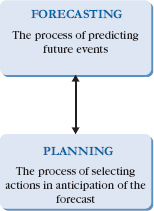
Forecasting is the process of predicting future events. This can range from forecasting product demand, such as demand for purple-colored ketchup in October, to forecasting the passage of a healthcare bill in Congress. Any time we try to predict future events we are forecasting. Planning, on the other hand, is the process of selecting actions in anticipation of the forecast. The forecast drives the plan and the plan is made in response to the forecast. This is shown in Figure 8.1.

Forecasting is one of the most important business activities because it drives all other business decisions. Decisions such as which markets to pursue, which products to produce, how much inventory to carry, and how many people to hire are all based upon a forecast. Consider the example of Nike in the chapter opener. The company continuously makes forecasts of demand for its many products and, as a result, generates plans regarding which products to produce and how much inventory to carry. Nike's poor forecasting, as a result of over reliance on forecasting software, resulted in incorrect business decisions. A similar situation occurred with the Goodyear Tire & Rubber Company a few years earlier. After investing in a state-of-the-art forecasting software the company did not achieve the anticipated forecast accuracy, resulting in high safety stock and too much inventory. As we can see, forecasting is a challenge. Also, poor forecasts result in poor planning and can leave the company unprepared to meet future demands. The consequences can be costly in terms of lost sales or excess inventory that cannot be sold.

Planning is the process of taking action in order to be prepared for the future. It requires organizing resources in anticipation of the forecast and being prepared for future events. As organizations attempt to decrease their vulnerability to chance they need to forecast and plan their resources accordingly. Forecasting and planning have become especially important as the lag time between awareness of an impending event and the need to respond have become increasingly short. The shorter this lag time the more critical forecasting and planning become.

FIGURE 8.1 Forecasting drives planning.

Planning involves the following decisions:

1. Scheduling existing resource. For a business and its supply chain to be competitive it must use its current resources in the most efficient way possible. This includes the production process, transportation, labor, facilities, and capital. An important aspect of planning is deciding how to best utilize existing resources.
2. Determining future resource needs. In addition to efficiently utilizing current resources, organizations must determine what resources are going to be needed in the future. These decisions depend on forecasts of emerging market opportunities, new technology, new products, and competition.
3. Acquiring new resources. It takes time for companies to acquire new facilities, new technologies, new equipment, or expand to new locations. Plans must be made well in advance, and procedures to acquire new resources and capabilities put in place well ahead of time.

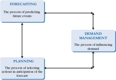
Companies often confuse forecasting and planning. The reason is that companies have the ability to affect demand. This can be done through promotional campaigns and advertisements, offering incentives to sales staff and personnel, and by cutting prices. This is called demand management and is the process of influencing demand.

Notice that demand management cannot occur without first having a forecast or a prediction of what future demand is going to be. Once a forecast and a resulting plan have been made, the organization may decide to influence demand in order to better utilize its resources, and the plan reconfigured accordingly. This is shown in Figure 8.2.

FIGURE 8.2 Forecasting, planning, and demand management.

IMPACT ON THE ORGANIZATION

Plans at all levels of the organization, from the strategic level where long-range plans are made, to the tactical where day-to-day scheduling is made, are based on forecasting. Also, forecasting drives the decisions of every organizational function. Marketing relies on forecasting to develop estimates of demand and future sales. Marketing also forecasts sizes of markets, new competition, future trends and emerging markets, and changes in consumer preferences. Finance, in turn, uses forecasting to assess financial performance and capital investment needs, to predict stock prices and investment portfolio returns, and set budgets. Operations makes decisions regarding production and inventory levels, conducts capacity planning and scheduling, all based upon a forecast. Sourcing uses forecasts to make purchasing decisions and select suppliers. None of these organizational functions could do their job without a forecast of the future. Whether in business, industry, government, or in other fields such as medicine, engineering, and science, proper planning for the future starts with a forecast.

IMPACT ON SUPPLY CHAIN MANAGEMENT

The forecast of demand is critical not only to the organization but to the entire supply chain, as it affects all the plans made by each company in the chain. When members of the supply chain make their forecasts independent of one another, they are only looking at the demand of their immediate buyer not the final customer in the chain. The consequences are a mismatch between supply and demand because each member of the chain is working to fulfil a different level of demand.

Consider the forecasting and planning process of Dell and Intel, one of Dell's suppliers. Dell starts its planning process with a forecast of future demand that is used to determine order quantities. At the same time, Intel, who supplies Dell with microprocessors, needs to determine its production and inventory schedules. If Dell and Intel were to make their forecasts independently of one another, their forecasts would differ and Intel would not be able to supply Dell with the exact quantities of microprocessors it needs. The best alternative is for Dell and Intel to collaborate. When there is collaboration between suppliers and manufacturers in generating the forecast, all entities are responding to the same level of demand.

Independent forecasting by members of the supply chain gives rise to the bullwhip effect, which we discussed in Chapter 1. The bullwhip effect refers to the increased volatility in orders as they propagate through the supply chain. The bullwhip effect occurs when each individual company in the supply chain forecasts its own demand, plans its stocking levels, and makes its replenishment decisions independently of other companies in the chain. This creates volatility in orders which makes forecasting more difficult, leads to increases in inventory throughout the supply chain, has a higher stock-out risk, and results in inefficient use of working capital and production capacity.

As we can see, forecasting has an impact on all organizations in the supply chain. The answer to good forecasting, and mitigating the bullwhip effect, is the sharing of data with supply chain partners and jointly generating forecasts.

Adapted from: “Lessons from the Pandemic That Wasn't.” Business Week, February 15, 2010.

THE FORECASTING PROCESS

PRINCIPLES OF FORECASTING

There are principles of forecasting that hold true regardless of what is being forecast. Let's look at these briefly.

1. Forecasts are rarely perfect. A perfect forecast is rare as there are too many factors in the business environment that cannot be predicted with certainty. Forecasting the future involves uncertainty and forecasters know that they have to live with a certain amount of error, which is the difference between the forecast and what actually happened. It is easy then to wonder why we should bother with forecasting. Although we may not achieve a perfect forecast, we can maintain overall good forecast accuracy.
2. Forecasts are more accurate for groups than for individual items. When items are grouped together, such as in product groups or families of items, their individual high and low values cancel each other out. The data for a group of items can be stable even when individual items in the group are unstable. The result is that higher degrees of accuracy can be obtained when forecasting for a group rather than for individual items. Consider Frito-Lay, a division owned by PepsiCo Inc., which owns brands such as Lay's Potato Chips, Fritos, Doritos, Ruffles, Sun Chips, and other brands. Frito-Lay can expect to have much lower forecast accuracy when forecasting demand for one specific product line, such as Baked Lay's potato chips, versus forecasting demand for all chips combined.
3. Forecasts are more accurate for shorter than longer time horizons. The shorter the time horizon of the forecast, the lower the degree of uncertainty. Data do not change much in the short run. As the time horizon increases, however, there is a much greater likelihood that changes in established patterns and relationships will occur. For that reason long-range forecasting tends to be less accurate than short range. For example, it is more difficult to forecast the size of an emerging market in Europe two years from now, than the size of the mobile phone market in Europe next month.

STEPS IN THE FORECASTING PROCESS

Forecasts need to be credible to be accepted by others. To ensure credibility there are some basic steps that should be followed when making a forecast, regardless of what is being forecast or the model used. The steps are as follows:

1. Decide what to forecast. This step may seem overly simple but it actually requires a bit of thought. For example, do we want to forecast actual sales versus total demand? Remember that forecasts are made in order to help plan for the future. To do so, we have to decide what forecasts are actually needed to guide the plan.
2. Analyze appropriate data. This step involves analyzing available data and identifying patterns present. There are patterns that can be observed in the data, although not every set of data has every pattern. It is important to identify which patterns are present and—in the next step—select the forecasting model most appropriate for that pattern. The most common data patterns are:
   1. Level or horizontal. This is the simplest pattern and exists when data fluctuate around a constant mean. It is the easiest to predict and is common for commodity products in the mature stage of the life cycle, such as table salt or toothpaste.
   2. Trend. Trend is present when data exhibit an increasing or decreasing pattern over time. The simplest type of trend is a straight line, or linear trend. However, a trend can take other forms, such as an exponential trend.
   3. Seasonality. Seasonality is any pattern that regularly repeats itself. Most of us think of ice cream sales in the summer or snow shovels in the winter. However, any pattern that regularly repeats itself is a seasonal pattern, such as restaurant sales that peak on the weekend.
   4. Cycles. Cycles are patterns created by economic fluctuations. Examples include recessions, inflation, or even the life cycle of a product. The major distinction between seasonality and cycles is that cycles do not have a predictable or repeating length or magnitude. As a result they are most difficult to predict.

   In addition to these patterns, data contain random variation that cannot be predicted. The more random variation in the data, the harder it is to forecast. Forecasting focuses on the patterns in the data, knowing that the random variation will be present. This is shown below:

   

3. Select the forecasting model. Once data patterns have been identified, the next step is to select an appropriate forecasting model. It is important to select the forecasting model best suited for the identified data pattern. Often we narrow the choice to two or three different forecasting models then test them on historical data to see which one is most accurate. We will look at specific models later in this chapter.
4. Generate the forecast. Once a model has been selected, the forecast is generated.
5. Monitor forecast accuracy. After the forecast has been made and actual events occur it is critical to evaluate forecast performance by measuring forecast error. This information should be used to improve the forecasting process. Remember that forecasting is an ongoing process that is always changing as new information and data become available.

FACTORS IN METHOD SELECTION

Someone new to forecasting might be overwhelmed by the choices in available forecasting methods. However, not all methods are appropriate for all forecasts. There are a few factors that should be considered in method selection:

1. Amount and type of available data. Different forecasting methods require different types and quantities of data. Sophisticated quantitative models, for example, may require large amounts of data, whereas simpler methods may not. In some cases—such as when forecasting new products—no historical data may be available. This factor plays a key role in the forecasting method that can be selected.
2. Degree of accuracy required. Sophisticated quantitative models may generate good forecasts but they may be costly to develop. The costs of the forecasting method need to justify the importance of the forecast. For example, forecasting paper clips or rubber washers doesn't justify a costly method of forecasting.
3. Length of forecast horizon. Some forecasting methods are better suited for short term forecasts, whereas others are better suited for long term. It is important to select the method most appropriate for the horizon being forecast. For example, forecasting emergency room visits at a hospital during the month of December is going to require a very different forecasting method than forecasting demand for natural gas over the next ten years.
4. Patterns in the data. As we already mentioned, it is critical to select a forecasting model that is appropriate for the identified patterns in the data. Otherwise, we can be guaranteed a poor forecast. For example, trying to forecast a product with a known trend pattern using a forecasting method that cannot capture trend will ensure errors.

Adapted from “A Different Game: Information is Transforming Traditional Businesses.” The Economist, February 28, 2010, pp. 6–7.

TYPES OF FORECASTING METHODS

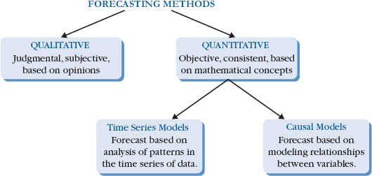
Forecasting methods can be classified into two broad groups: qualitative and quantitative. They are shown in Figure 8.3.

Qualitative forecasting methods, often called judgmental methods, are methods based on subjective opinions and judgment of individuals, such as managers, sales staff, or customers. Asking customers whether they would buy a particular product, called “intention surveys,” is a type of qualitative forecasting method. Another one is called “sales force composite” and occurs when the sales staff make a group forecast of upcoming sales. Qualitative methods are made by people and, as a result, are subject to human biases.

Quantitative forecasting methods, on the other hand, are based on mathematical modeling. These methods are objective and consistent, are capable of handling large amounts of data and uncovering complex relationships. Provided that good data are available, these methods are generally more accurate than qualitative methods.

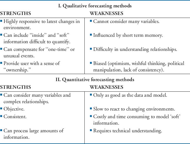
Both qualitative and quantitative forecasting methods have their strengths and weaknesses, as shown in Figure 8.4. Although quantitative methods are objective and consistent, they require data in quantifiable form in order to generate a forecast. Often, such data is not available, such as in new product forecasting or making long-range strategic forecasts. Also, quantitative methods are only as good as the data on which they are based. Qualitative methods, on the other hand, have the advantage of being able to incorporate last minute “inside information.” This may be last minute notice of a competitor's advertising campaign, a snowstorm delaying a shipment, or a heat wave increasing ice cream sales. Each method has its role in the forecasting process and a good forecaster learns to rely on both.

QUALITATIVE FORECASTING METHODS

There are numerous qualitative forecasting methods, ranging in degree of formality and structure. These methods are especially useful when identifying customer buying patterns, expectations, and providing sales estimates of new products.

FIGURE 8.3 Categories of forecasting methods.

FIGURE 8.4 Qualitative versus quantitative forecasting methods

Executive opinion is a type of qualitative forecasting method where a group of managers, executives, or sales staff meet and collectively develop a forecast. This method is often used to forecast sales, market trends, make strategic forecasts, or forecast new products. Also, it can be used to modify existing forecasts to account for special events, such as slowed spending during a recession or a special promotional campaign.

The advantage of this method is the ability to include the latest information in the forecast. The disadvantage, however, is that it is subject to many human biases, such as optimism, inconsistency, and political manipulation. Also, because it is a group decision-making process, often the opinion of one member can dominate the forecast.

Market research uses surveys and interviews to determine customer likes, dislikes, and preferences, and to identify new product ideas. Conducting market research requires understanding how to conduct reliable surveys. Therefore, companies usually hire an outside marketing firm to conduct a market research study.

Market research can be a good determinant of customer preferences. However, it has a number of shortcomings. A common one is the potential inadequacy of the survey questionnaire design. For example, a market research firm may ask participants to identify a favorite hobby providing them with the following choices: gardening, fishing, cooking, or sports. The problem in this example is that the list is not exhaustive, as a participant may prefer music—an option not included. This questionnaire forces participants to select a category. As a result, the findings will incorrectly portray customer preferences and lead to misinterpretation of the market.

The Delphi method is designed to reach a consensus among a group of experts on a particular topic. Examples may include forecasting propagation of a disease, climate changes, or technological innovation. The process involves choosing experts in the field of inquiry, who maintain anonymity. Questionnaires are sent to the experts, the findings summarized, and the process repeated with updated questionnaires that incorporate the initial findings. This process continues until consensus between the experts is reached.

Delphi is based on the assumption that although experts in a field typically do not agree on many things, what they do agree on will likely happen. The researcher's job is to extract this information. Although it is time consuming, Delphi has been shown to be an excellent method for forecasting long-range product demand, technological change, and scientific advances in medicine.

QUANTITATIVE FORECASTING METHODS

Unlike qualitative methods that are based on opinions, quantitative methods are based on mathematical concepts. Quantitative methods can be divided into two broad categories: time series and causal models, as shown in Figure 8.5. Although both are mathematical, the two categories differ in their assumptions and how the forecast is generated.

Time series models generate the forecast from an analysis of a “time series” of the data. A time series is simply a listing of data points of the variable being forecast over time taken at regular intervals. For example, data of student enrollment per semester at a university over the past five years is an example of a time series. Time series models assume that forecasts can be made by identifying and modeling the patterns present in the data.

FIGURE 8.5 Categories of quantitative forecasting methods.

Causal models assume that the variable being forecast is related to other variables in the environment. For example, university enrollment may be related to unemployment rates, recession levels, or salary levels. In this case the forecasting process involves identifying these relationships, expressing them in mathematical form, and using that information to generate a forecast.

Time series models are generally easier to use than causal models. They are also more readily available in forecasting software. Causal models, on the other hand, can be more complex, especially if relationships between multiple variables are being considered. However, time series models can often be just as accurate and have the advantage of simplicity. They are easy to use and can generate a forecast more quickly than causal models, which require model building. For this reason, time series models are used more frequently in environments where large numbers of items must be forecast on a regular basis, such as retail. Recall the many different products that must be forecast at Nike. Time series analysis would likely be best for that large variety of items.

TIME SERIES FORECASTING MODELS

THE MEAN

One of the simplest forecasting models is the mean, where the forecast is made by simply taking an average of all the data:

where

This method is only appropriate for a level data pattern. It is, however, a reasonable forecasting model to use for forecasting stable and mature products. One advantage of this method is that as more data is collected over time, and the average becomes based on a larger data set, the forecasts become more stable.

Example Forecasting with the Mean

Handy Power Tools is forecasting sales of its most popular drill. The company has been selling the drill for the past 15 years and sales have been steady. The company uses a simple mean to forecast weekly sales. Sales over the past five weeks are available and the company will use them to make a forecast for week six.

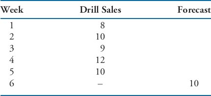
The forecast is simply an average of the past five weeks:

MOVING AVERAGES

The simple moving average is a method that generates a forecast by averaging a specified number, n, of the most recent data rather than the entire data set. As new data become available, the oldest are dropped, and the number of observations used to compute the average is kept constant. In this manner, the simple moving average “moves” through time. Like the mean, this model is only appropriate for level data patterns. However, it does have the advantage of being responsive by averaging only the most recent observations.

The formula is as follows:

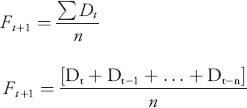
where

Notice that n is not the entire data set but only a subset of the data used in the average. For example, if n=3 the average would include only the latest three data points. If n=5 the average would include only the latest five data points, and so on. In general, the more data points that are used in the average the more stable the forecast as more data is being averaged. On the other hand, the fewer the data points in the average the more responsive the forecast.

Example Forecasting with the Simple Moving Average

La Petite Tableau forecasts sales of kitchen aprons using a three-period moving average. How many aprons should they expect to sell in April given the following sales figures for January, February, and March?

Month	Actual sales
January	38
February	27
March	42

To find the forecast for April we take an average of the last three observations:

If La Petite Tableau sells 42 aprons in April, let's make a forecast for May continuing to use a three-period moving average.

Notice that in a simple moving average all the data are weighed equally, that is 1/n. Sometimes we may want to give more or less weight to certain data points, such as giving more weight to recent observations. This is called a weighted moving average. The computation is the same except that managers have the option of specifying the weights assigned to the data point.

EXPONENTIAL SMOOTHING

Exponential smoothing is a forecasting model that uses a special weighted average procedure to obtain a forecast. It is easy to use and understand, and provides good forecast results. To make a forecast just three items are needed:

1. current period's forecast
2. current period's actual value
3. value of a smoothing coefficient, α, which varies between 0 and 1.

The equation for the forecast is:

where

Example Forecasting with Exponential Smoothing

Cafe Nervosa uses exponential smoothing to forecast monthly usage of coffee cream. Its forecast for May was 24 gallons, but the actual usage turned out to be 28 gallons of coffee cream. The manager has chosen to use an alpha of 0.70. What is her forecast for June?

Using the exponential smoothing equation

The critical aspect of exponential smoothing is selecting a correct value for α. High values of α place more weight on current period's actual demand, whereas low values place more weight on the current period's forecast. Values of α that are low say, 0.1 or 0.2, generate forecasts that are stable as more weight is placed in historical data and less on the current period's actual demand. However, these forecasts are less responsive to recent changes in demand. Values of α that are high, say, 0.7 or 0.8, place a large weight on the current period's actual demand. As a result, they generate forecasts that are responsive to latest changes in demand, but can be less stable.

When using exponential smoothing for the first time we may not have a forecast for the current period. The most common way to handle this is to use what is called “the naive method”, which is using last period's actual value to generate an initial forecast. Another option is to average the last few periods—say the last three or four—just to get a starting point.

TREND ADJUSTED EXPONENTIAL SMOOTHING

The models discussed so far work only for a level pattern. If there is a trend in the data the models need to be modified, otherwise the forecasts will “lag” the trend. One of the more common ways to forecast trend is to use trend adjusted exponential smoothing. It is a simple modification of the exponential smoothing model we just discussed. The model takes the basic exponential smoothing equation and just adds a trend component to compensate for the additional pattern:

where

To generate a forecast including trend, FIT_t+1, we need to follow these steps:

• Step 1 Generate an unadjusted forecast FIT_{t + 1}
• Step 2 Generate trend T_{t + 1} (notice that F_t feeds into the trend equation)
• Step 3 Add F_{t + 1} and T_{t + 1}

Example Forecasting with Trend Adjusted Exponential Smoothing

Looking at the following data assume that we are at the end of January and want to forecast one period ahead using trend adjusted exponential smoothing. We have decided to use an α = 0.3 and a β = 0.4. Assume that we are rolling through time knowing the actual demand after we have made the forecast, and using the information to forecast the subsequent period.

How did we get the above numbers? Let's follow the steps to generate the forecast for February.

• Step 1 Generate an unadjusted forecast F_t+1

  

• Step 2 Generate trend T_t+1 (notice once again that F_t feeds into the trend equation)

  

• Step 3 Add F_t+1 and T_t+1

  

The other numbers in the table are obtained in the same manner. Notice the difference in the unadjusted versus adjusted forecast. How different do you think the adjusted values would be with a different value of β?

SEASONALITY ADJUSTMENT

Seasonality is any regularly repeating pattern. Consider sales of ice cream in the summer or snow shovels in the winter, university enrollment in the fall, amusement park attendance in the summer, or sales of turkeys at Thanksgiving.

When seasonality is present we need to adjust our forecast to reflect the amount by which the particular “season” is above or below the average. This is estimated as a percentage, such as saying that amusement park attendance is 140% of the average during the month of June, whereas it is 70% of the average in March. This percentage is called the seasonal index. Adjusting for seasonality simply involves computing the seasonal index—or percentage—and using it to adjust the forecast. This is detailed in the following steps:

• Step 1 Compute average demand for each “season.” Total annual demand is divided by the number of “seasons” per year. For quarterly data the number of “seasons” would be 4, whereas for monthly data it would be 12.
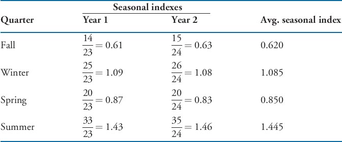
• Step 2 Compute a seasonal index for each season. A seasonal index is obtained by dividing the actual demand for each season by the average demand for each year. An average seasonal index is then obtained by averaging across the number of years available.
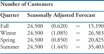
• Step 3 Adjust the average forecast for next year by the seasonal index. Generate a forecast for next year using any of the methods we discussed and calculate average demand per season. Use seasonal indexes to generate seasonally adjusted forecasts.

Example Generating Seasonally Adjusted Forecasts

Coco's Ice Cream Shop experiences high seasonality in customer sales. It sells ice cream throughout the year, with most sales occurring in the summer; it also sells hot chocolate, with most sales occurring in the winter. Coco has generated a forecast for next year to be 98,000 customers. Use the data below to create a seasonally adjusted forecast per quarter.

Solution:

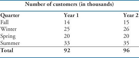
Step 1 Compute average demand for each “season.”

Step 2 Compute a seasonal index for each season.

Step 3 Seasonally adjust the average forecast for next year.

The forecast for next year is 98,000, so the average demand is 24,500.

CAUSAL MODELS

LINEAR REGRESSION

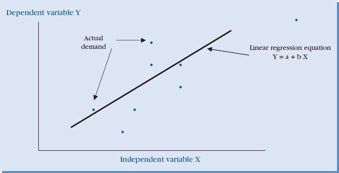
Linear regression is a forecasting model that assumes a linear, or straight line, relationship between two variables. It assumes that the variable being forecast, called the dependent variable, is linearly related to another variable, called the independent variable. For example, if we assume that a person's weight and height are linearly related, we can create a linear regression model of this relationship. We can then use the model to forecast weight based on a person's height. It is also possible to use time as the independent variable if we want to see how a variable changes over time. In this case it could be used to forecast trend.

Linear regression is a method that fits a straight line through a set of data, as shown in Figure 8.6. You can see that the dependent variable is linearly related to the independent variable. The relationship between two variables is the equation of a straight line as follows:

FIGURE 8.6 Linear regression line.

where

• Y = dependent variable
• X = independent variable
• a = Y intercept of the straight line
• b = slope of the straight line

Using linear regression requires first developing the linear regression equation. Then for any value of the independent variable we can compute the value of the dependent variable, which is the variable being forecast. The steps involved are as follows:

• Step 1 Compute parameter b:

  

  where

  

• Step 2 Compute parameter a:

  

• Step 3 Substitute values for a and b in the equation:

  

• Step 4 Generate a forecast for the dependent variable (Y). Substitute the appropriate value for the independent variable (X).

Example Forecasting with Linear Regression

Pizza Boy is trying to forecast the volume of pizza sold based on the amount of money it has put into advertising in the local newspaper. It has been tracking the relationship between pizza sales and advertising over the past four months. The results are as follows:

Pizza Sales	Advertising Dollars
58	135
43	90
62	145
68	145

What would happen to pizza sales if Pizza Boy invested $150 in advertising for next month?

In this example pizza sales are the dependent variable (Y) and advertising dollars the independent variable (X). Following the outlined steps we formulate the following table:

From the above we compute and

• Step 1 Compute parameter b:

  

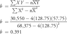
• Step 2 Compute parameter a:

  

• Step 3 Substitute values for a and b in the equation:

  

• Step 4 Generate a forecast for the dependent variable (Y). Substitute the appropriate value for the independent variable (X).

  

MULTIPLE REGRESSION

Multiple regression extends linear regression by looking at a relationship between the independent variable and multiple dependent variables. The general formula for multiple regression is as follows:

where

For example, the dependent variable might be university student enrolment per semester and the independent variables might be unemployment rate and per capita income. Other variables that can be included are seasonality and trend, as well as special events such as promotions that can be included as separate variables. Multiple regression is a powerful tool for forecasting. The drawback, however, is that it has increased computational and data requirements.

MEASURING FORECAST ACCURACY

Measuring forecast accuracy is a critical aspect of forecasting. This tells us how our forecasting methods are performing and enables us to improve performance over time. Data can change over time and models that once provided good results may no longer be adequate. The model's accuracy can be assessed only if forecast performance is measured over time.

The first step in measuring forecast accuracy is to measure the forecast error. Forecast error is the difference between actual demand and the forecast for a given period:

where

However, computing error for one time period does not provide enough information. We need to measure forecast accuracy over time. Two of the most commonly used error measures are the mean absolute deviation (MAD) and the mean square error (MSE). MAD is the average of the sum of the absolute errors:

MSE is the average of the squared error:

Both of these measures are useful and provide the forecaster with different information. An advantage of MAD is that it is based on absolute values. As a result, errors of opposite signs do not cancel each other out when they are added, providing a total sum of the average error. When comparing different forecasting methods we would select the method with the lowest MAD.

MSE has an additional advantage. Due to the squaring of the error term large errors are magnified, giving them greater penalty. This can be a useful error measure in environments where large errors are particularly destructive. As with MAD, when comparing the forecast performance of different methods we would select the method with the lowest MSE. Both error measures provide different information and a good forecaster learns to rely on multiple measures.

Example Measuring Forecast Accuracy

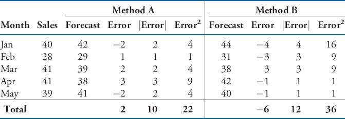
Harry Thurber (HT) Apparel is comparing the accuracy of two methods that it has used to forecast monthly sales of its popular jeans. Forecasts of monthly sales from January through May for method A and method B are shown below against the actual sales. Which method provided better forecast accuracy?

Accuracy for method A:

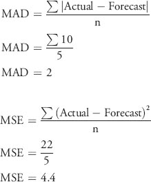
Accuracy for method B:

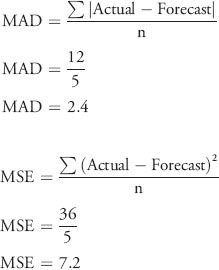
Of the two methods, method A produced both a lower MAD and a lower MSE, which means that it provided better forecast accuracy.

COLLABORATIVE FORECASTING AND DEMAND PLANNING

Forecasting is most effective when it is done in collaboration with supply chain partners. In this section we look at two of the most common processes for collaborative forecasting and demand planning.

COLLABORATIVE PLANNING, FORECASTING AND REPLENISHMENT (CPFR)

Collaborative Planning, Forecasting, and Replenishment (CPFR) is a collaborative process of developing joint forecasts and plans with supply chain partners, rather than doing them independently. It is based on the premise that companies can be more successful if they work together to bring value to their customers, share risks of the marketplace, and improve their performance. CPFR was developed by the Voluntary Interindustry Commerce Standards (VICS) association, a non-profit organization formed in l986 to develop standards and guidelines for improving supply chain efficiency. CPFR is one such set of guidelines and provides a process to be followed in achieving coordination for both forecasting and inventory replenishment.

VICS membership includes major corporations such as Wal-Mart and P&G. These companies have demonstrated the benefits that can be achieved with CPFR. The organization has a specific “CPFR committee,” which offers detailed guidelines on how supply chain members can collaborate to improve efficiency. The guidelines are based on standard technologies and are scalable, enabling ready implementation across different industries.

The distinguishing feature of CPFR is that members of the supply chain collaborate on business plans, and jointly execute the processes of forecasting and replenishment. Trading partners jointly set forecasts, plan production, replenish inventories, and evaluate their success in the marketplace.

The benefits of CPFR are impressive and it has been implemented by many companies, including Wal-Mart, Target, Black & Decker, and Ace Hardware. In 2001 an AMR Research study found that by implementing CPFR retailers and suppliers jointly achieved higher sales, decreased inventory, improved stock levels, while lowering their logistics cost. Similarly, Kurt Salmon Associates estimated the benefits from CPFR on the apparel industry as roughly being $8.3 billion annually (www.vics.org).

VICS offers a five-step process for adoption of CPFR:

• Step 1 Create joint objectives.
• Step 2 Develop a business plan (e.g., forecasting needs, production schedules, key performance metrics, or “KPIs”).
• Step 3 Create a joint forecast.
• Step 4 Agree on replenishment strategies.
• Step 5 Agree on a technology partner to bring CPFR to fruition.

Although these steps seem simple they can often be difficult to implement as they require companies to trust each other, and be flexible and willing to work together. It should also be pointed out that CPFR is not a one-time event. Rather it is an ongoing process where the outlined steps are performed on a weekly or monthly basis, and the agreement between parties is evaluated annually.

SALES AND OPERATIONS PLANNING (S & OP)

In Chapter 2 we discussed that sometimes organizational functions—such as marketing and operations—operate independently of one another, resulting in overall poor performance. An organization can have several functional forecasts for the same products over the same time period, such as a financial forecast, an operations forecast, a marketing forecast, and a distribution forecast. As these functional forecasts are made independently of one another they typically do not agree. For example, marketing may forecast demand for products that neither manufacturing nor distribution can meet. For an organization to develop efficient and realistic plans for the future, it must generate forecasts that all functional areas agree upon and can execute.

Adapted from: “A Different Game: Information is Transforming Traditional Businesses.” The Economist, February 28, 2010: 6–7.

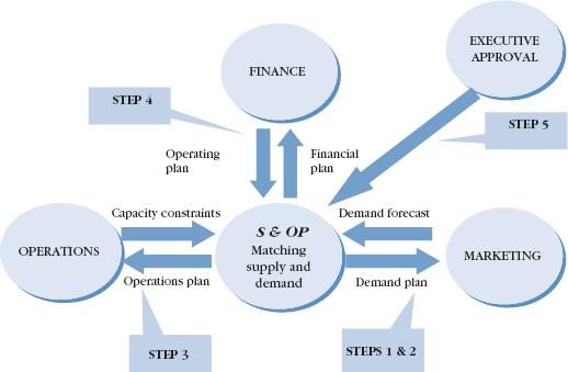
Sales and Operations Planning (S & OP) is an organizational process intended to match supply and demand through functional collaboration. S & OP requires teamwork among sales, distribution and logistics, operations, finance, and product development. This enables firms to provide better customer service, lower inventory, reduce customer lead times, and stabilize production schedules. The process is designed to coordinate activities between marketing and sales, with those of operations and sourcing, in order to ensure that supply meets demand requirements.

The S&OP process consists of a series of meetings with the goal of reaching an agreement between various departments on the course of action to achieve the optimal balance between supply and demand. It consists of a five-step process that needs to be followed to arrive at a consensus forecast:

• Step 1: Generate quantitative sales forecast. This process is done using one or more of the forecasting techniques discussed in the previous section.
• Step 2: Marketing adjusts the forecast. These adjustments include promotions of existing products, introduction of new products, or the elimination of products. This revised forecast is usually stated in terms of both units and dollars.
• Step 3: Operations checks forecast against existing capability. This includes an evaluation of whether existing capacity is adequate to handle the forecasted volumes. Operations must analyze availability of resources, such as inventory, production capacity, scheduling, and labor, for meeting overall demand and “spike” demand. This may signal the need for extra resources to support special promotions.
• Step 4: Marketing, operations, and finance jointly review forecast and resource issues. This is a joint meeting of the key business functions to review the forecast and any capacity issue that might have emerged during step 3. During this phase attempts are made to solve capacity issues and balance supply and demand. Alternative scenarios are usually developed and considered, identifying potential lost sales and costs associated with each scenario. At this stage the forecast is converted to dollars to assess whether the scenarios meet the financial plan of the organization.
• Step 5: Executives meet to finalize forecast and capacity decisions. At this meeting executives from each functional area meet to make final decisions regarding sales forecasts and capacity issues. Executives reach agreement on the forecast and convert it into the operating plan for the organization.

FIGURE 8.7 The S & OP Process.

This process is illustrated in Figure 8.7.

S & OP is an important process as it forces functional agreement and creates an understanding of revenue and cost trade-offs. It also forces the joint plan to measure functional performance in terms of metrics appropriate for each functional area, enabling it to support the overall business plan. For example, let's say that performance of the operations function is measured on “cost per unit.” This metric encourages operations to keep costs low. A promotional campaign by marketing may mean higher per unit costs for operations, as it needs to extend its resources. These metrics for operations discourage it to support marketing. A better solution is to revise the metric for operations to something such as “compliance to schedule.” This new metric would reward operations for making the planned quantities at the planned times. This is an example of what could be achieved through S & OP. S & OP encourages functions to jointly work together to achieve goals of the business plan.

CHAPTER HIGHLIGHTS

1. Forecasting is the process of attempting to predict future events. Planning is the process of selecting actions with the hope that they will result in attainment of goals and objectives given the forecast.
2. There are three principles of forecasting: (a) forecasts are rarely perfect; (b) forecasts are more accurate for aggregated items than for individual items; and (c) forecasts are more accurate for shorter than longer time horizons.
3. Data are composed of pattern and randomness. Four of the most common patterns are level, trend, seasonality, and cycle.
4. Forecasting methods can be divided into qualitative and quantitative. Qualitative methods are subjective and based on opinions. Quantitative methods are mathematically based, are objective and consistent.
5. Quantitative forecasting methods can be divided into two categories: time series and causal models.
6. Time series models generate the forecast by identifying and analysing patterns in a “time series” of the data. Causal models assume that the variable being forecast is related to other variables in the environment and develop a model identifying these relationships, expressing them in mathematical terms, and using that information to forecast the future.
7. CPFR is a collaborative process of developing joint forecasts and plans with supply chain partners, rather than doing them independently.
8. Sales and Operations Planning (S & OP) is an organizational process intended to match supply and demand through functional collaboration between marketing, operations, and finance, in order to ensure that supply can meet demand requirements.

KEY TERMS

• Forecasting
• Planning
• Demand management
• Qualitative forecasting methods
• Quantitative forecasting methods
• Executive opinion
• Market research
• The Delphi method
• Time series models
• Causal models
• Simple moving average
• Weighted moving average
• Seasonal index
• Linear regression
• Multiple regression
• Collaborative Planning, Forecasting, and Replenishment (CPFR)
• Sales and Operations Planning (S & OP)

DISCUSSION QUESTIONS

1. Identify a nontraditional business event, such as forecasting demand for t-shirts following the Super Bowl, or the amount of relief aid needed following an earthquake. What do you think would be the best way to forecast such an event—qualitative or quantitative—and why? What are the implications of forecast error on supply chain management?
2. Think of a product you have recently purchased. How many different forecasts do you think the retailer had to make in order to decide how much product to stock? What are the consequences for that particular retailer if they had over forecast versus under forecast?
3. Imagine that you are starting a business. What type of forecasting model would you use to decide how many products you will be selling? Would you use the same forecasting model after you have been in business five years? Why or why not?
4. Identify an example where large errors would be extremely costly. Which forecast error metric would be best for this environment?
5. Identify the differences between the two methods of collaboration discussed in the chapter: CPFR and S & OP. How are they similar and how are they different? Explain the differences in the organizational objectives they are trying to achieve.

PROBLEMS

1. Beyond Tea Inc. wants to forecast sales of its menthol green tea. The company is considering either using a simple mean or a three-period moving average to forecast monthly sales. Given sales data for the past 10 months use both forecasting methods to forecast periods 7 to 10 and then evaluate each. Which method should they use? Use the selected method to make a forecast for month 11.

   Month	Sales (lbs)
   1	5
   2	8
   3	15
   4	18
   5	20
   6	19
   7	17
   8	18
   9	19
   10	21

2. Safe Spirit sells novelty hats in New York City. The company uses a simple mean to forecast monthly sales. The forecast of sales for month six was $5,000 obtained by averaging past 5 months' sales. Sales from months one to four were: $6,000, $7,000, $4,000, and $5,000. However, the sales assistant accidently deleted the sale data for month five in the system. Now, the sales manager wants to determine sales for month five from the remaining data. How would she do that?
3. Mr. Zhou repairs computers. He had 45 customers for January, 50 customers for February and 70 for March. He now wants to forecast his customers for April by using a two-period simple moving average. Compute the forecast.
4. Smile Cucumber Corp records its sales in a database system. The company wants to forecast monthly sales based on the record of the past three months. The value of the forecast is 10 million if the company uses the simple mean. What is the forecast if the company uses a three-period moving average? Explain.
5. Green Water Park uses exponential smoothing to forecast monthly visits of customers. Its forecast for June was 1 million, but the actual number of customers turned out to be 2 million. The forecaster decided to use an alpha of 0.8. What is the forecast for July?
6. Katherine is a forecast manager. She used exponential smoothing to forecast her sales of coffee cakes for next week and this number is 200. Her forecast for this week was 180 but the actual number is 220. What is her choice for alpha?
7. The past two years sales at ACSR Inc. were 2 million and 4 million. Their forecast team used a two-period moving average to forecast its sales this year. But the actual sales for this year were 4 million. Now, the forecast team wants to forecast its sales for next year by using exponential smoothing with alpha equals 0.7. What is the forecast?
8. Gold Roof Hut is trying to forecast its number of customers based on the average price of food. It has been tracking the relationship between number of customers and food's average price over the past five weeks. The results are as follows:

   Number of customers (in thousands)	Average price (in dollars)
   1	16
   1.2	15
   1.4	14
   1.8	12
   1.8	11

   What would be the number of customers if Gold Roof Hut set the average price to 10?

9. Alexandra is forecasting sales based on the salesperson's salary. She collected the following data and would like to forecast sales if salary is 6K:

   Sales (10 K)	Salary (K)
   1	2
   1.5	3
   2	3.5
   3	4
   3.2	5

10. Mixo Inc. is forecasting its product's quality on a scale of 0 to 100 based on how many hours are spent for each product. Data are in the following table:

    Quality	Hours spent
    50	10
    60	15
    70	20
    80	24
    90	30

    How many hours should be spent if the company wants its product quality to be 95?

11. John Taylor Salons wants to forecast monthly customer demand from June through August using trend adjusted exponential smoothing. Given α = 0.2, β=0.4, F _MAY=45, and a T_MAY=0, forecast a FIT for months June through August.

    Month	Actual sales
    May	50
    June	61
    July	73
    August	80

12. Henry Lo Manufacturing is comparing the accuracy of two methods that it has used to forecast monthly production. Forecasts of monthly productions from May through August are shown below against the actual productions. Which method provided better forecast accuracy?

    

13. Samuel Bridge Company wants to compare the accuracy of two methods that it has used to forecast yearly profits. Forecasts of yearly profits from 2006 through 2010 are shown below against the actual productions. Comment on their forecast accuracy.

    

14. Jay Sharp Guard wants to compare the accuracy of two methods that it has used to forecast monthly expenses. Forecasts of monthly expenses from September to November are shown below against the actual expenses. Which method provided best-forecast accuracy?

    

CASE STUDY: SPEEDY AUTOMOTIVE

It is August 2008 and Speedy Automotive is one of four car dealerships located in rural Wyoming. The residents in the area replace their vehicles roughly every eight years. When they do replace their vehicles, they tend to visit the same dealership that sold them the first one, building a relationship with the dealership. This has kept sales relatively stable for all the dealerships in the area. Recently, however, customers have begun expanding their shopping options. Speedy Automotive believes this is due to the rise of the Internet. Customers have begun coming to the dealership with an exact idea of what car they would like and have a price in mind. When Speedy Automotive does not have the model available or cannot meet the price, customers have started going to competitors.

This trend has the general manager of Speedy, Mike Leavy, worried. Mike runs the dealership like a small business and relies on repeat customers. Speedy is not a chain and has little access to outside capital, so cash flow is critical. If sales are low, Mike has to take out a loan to pay the manufacturer for the vehicles. If sales are high, Speedy loses potential customers due to lack of inventory. Mike has decided that he needs to be able to forecast this new variability to keep the business healthy.

Bill Goodson is the inventory manager at Speedy and has historically prepared the forecasts. Bill usually just takes the sales numbers from last year and adjusts them upward or downward based on his “gut feeling.” This has worked well in the past, but Mike has told him to look into other forecasting methods. Bill is preparing the September 2008 sales forecast for Speedy and is not sure where to start. For the August forecast, Bill used the sales numbers from August 2007. The August 2007 forecast was off by 10 cars and Bill hoped the 2008 version would fare better. Bill assumed the sales representatives would always work a little harder if sales were low and they could always take vacation time if they were above target.

Mike has told Bill to look into both time series and causal forecasting models, but Bill is not sure of the difference. Mike also wants Bill to determine the amount of profit being lost due to poor forecasting. Bill has access to sales and forecast data from the past 18 months and has already calculated various measures of error in Excel.

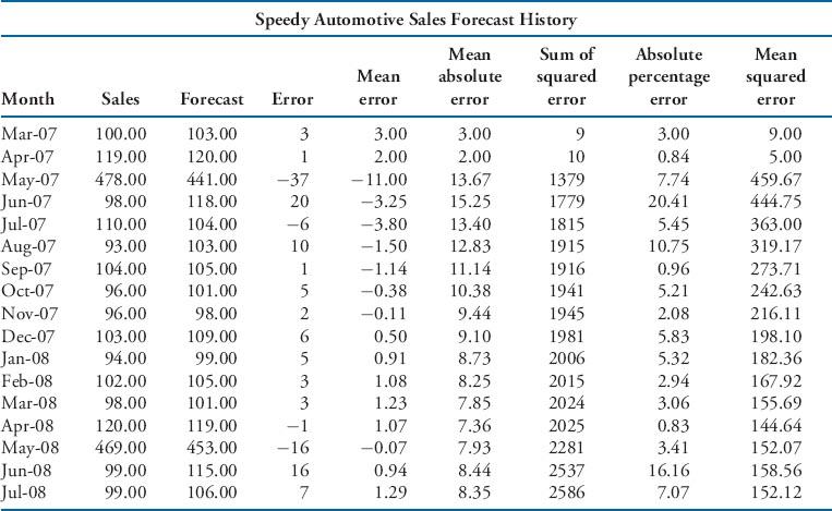
CASE QUESTIONS

1. Is Speedy Automotive currently using a time series or causal forecasting? Explain the difference and how you can identify each.
2. Is this type of forecast appropriate or would an alternative method produce more accurate results? Why or why not?
3. Which measure should Bill use to assess forecast error rates? Why?
4. If Bill's forecasts are consistently too high or consistently too low, which measure is most useful to remedy the situation? Why?
5. If the average sale price for one car is $20,000 and the average car costs $15,000 to acquire, how much profit is being lost each month as a result of poor forecasting? Note: For ease of calculation, assume all cars arrive on the 1^st and all cars remaining on the 31^st are disposed of with a 50% markdown.
6. What can Bill do to improve his forecasting based on your observations?

REFERENCES

Armstrong, J. Scott. Long-range Forecasting: From Crystal Ball to Computer. New York: John Wiley & Sons, 1985.

Armstrong, J. Scott, and Fred Collopy. “Error Measures for Generalizing about Forecasting Methods: Empirical Comparisons.” International Journal of Forecasting. 8, 1992: 69–80.

Boone, Tonya, and Ram Ganeshan. “The Value of Information Sharing in the Retail Supply Chain: Two Case Studies.” Foresight. Issue 9, Spring 2008: 12–17.

Collopy, F., and J. Scott Armstrong. “Rule-Based Forecasting: Development and Validation of an Expert Systems Approach to Combining Time Series Extrapolations.” Management Science. 38(10), 1992: 1394–1414.

Lee, H., V. Padmanabhan, and S. Whang. “The Bullwhip Effect in Supply Chains.” Sloan Management Review, 38(3), 1997: 93–102.

Makridakis, S., S. C. Wheelwright, and Rob J. Hyndman. Forecasting: Methods and Applications; 4th edition. New York: John Wiley & Sons, 2006.

Siems, T. F. “Supply Chain Management: The Science of Better, Faster, Cheaper.” Southwest Economy. Issue 2, March/April 2005: 6–12.