Chapter 9
Inventory Management
After completing this chapter, you should be able to:
- Describe different types of inventory, their uses and costs.
- Explain inventory systems and ordering policies.
- Understand how to compute order quantities, reorder points, and safety stock.
- Differentiate between independent and dependent demand.
- Understand practical issues of managing supply chain inventories.
- Explain ABC inventory classification and vendor managed inventory (VMI).
![]() Chapter Outline
Chapter Outline
- Basics of Inventory Management
What is Inventory?
Reasons for Carrying Inventory
Types of Inventory
Inventory Costs
- Inventory Systems
Fixed-Order Quantity System
Fixed-Time Period System
Comparing Fixed-Order Quantity Versus Fixed-Time Period Systems
- Fixed-Order Quantity System
The EOQ
Economic Order Quantity (EOQ)
Reorder Point (ROP)
Safety Stock
Economic Production Quantity (EPQ)
- Fixed-Time Period Systems
Computing Target Inventory
- Independent Versus Dependent Demand
- Managing Supply Chain Inventory
ABC Inventory Classification
Practical Considerations of EOQ:
Lumpy Demand (POQ)
EOQ Adjustments
Capacity Constraints
Measuring Inventory Performance
Vendor Managed Inventory (VMI)
- Chapter Highlights
- Key Terms
- Discussion Questions
- Problems
On an early July morning a crowd has gathered for the opening of Trader Joe's newest store location, in Manhattan's Chelsea neighborhood. As shoppers stand in line for the store's opening, they chat about their favorite Trader Joe's foods and discuss the benefits the store opening will bring to the area. Why the excitement? Trader Joe's is no ordinary grocery chain. It is offbeat and hip, having elevated food shopping to a cultural experience.
Trader Joe's has developed an almost cult following and is one of the hottest retailers in the United States, with 344 stores in 25 states and Washington, D.C. They see themselves as a national chain of neighborhood specialty stores, stocking shelves with a winning combination of low-cost, yuppie-friendly goods. This includes staples such as cage-free eggs and organic blue agave sweetener. They also carry the exotic, such as Belgian butter waffle cookies and Thai lime-and-chili cashews—items difficult to find anywhere else.
What is most remarkable about Trader Joe's is that they have found a unique way of addressing the problem that has traditionally plagued grocery stores: carrying large numbers of highly perishable food items in large varieties. A typical grocery store carries about 50,000 stock-keeping units (SKUs), while Trader Joe's carries about 4,000 SKUs. As a result, its stores sell an estimated $1,750 in merchandise per square foot, which is more than double that of Whole Foods. The company doesn't carry much inventory and has little back room space for storage. However, the inventory that it does carry is carefully selected.
Trader Joe's pursues a limited-selection, high-turnover inventory model. One example is peanut butter. Trader Joe's sells 10 varieties, compared to most supermarkets that sell about 40. This has huge implications for inventory turnover. Imagine that a typical supermarket and a Trader Joe's both sell 40 jars of peanut butter a week. Trader Joe's would sell an average of four of each type, while the supermarket might sell only one. With the greater turnover on a smaller number of items, Trader Joe's can buy large quantities with deep discounts. It also has lower losses due to shelf life. This makes operations—from stocking shelves to checking out customers— much simpler.
Customers accept Trade Joe's limited variety trusting that the company will stock only the best. For example, there are only two kinds of pudding or one kind of polenta. As one former employee puts it, “If they're going to get behind only one jar of Greek olives, then they're sure as heck going to make sure it's the most fabulous jar of Greek olives they can find for the price.”
Management has sought to minimize the number of hands that touch a product throughout the supply chain. Whenever possible, Trader Joe's buys directly from the manufacturer, which then ships the items straight to Trader Joe's distribution centers. For example, a U.S.-made cheese is sent to distribution centers nationwide, where it is cut and wrapped. At a traditional supermarket, that same cheese would typically go through a distributor first, adding another inventory cost to the supply chain. Trucks leave the distribution centers daily for the stores, which keep low inventory levels. Trader Joe's small stores don't have much of a back room so ordering from the distribution centers has to be precise. All this has kept costs low, enabling Trader Joe's to be in an enviable financial position: having no debt and self funding their growth.
Adapted from: “Inside Trader Joe's.” Fortune, September 6, 2010: 86–96.
BASICS OF INVENTORY MANAGEMENT
WHAT IS INVENTORY?
Simply put, inventory is quantities of goods in stock. This is true for any product, material, or good. Consider the books or CDs on your bookshelf. They comprise your inventory. They provide you with a certain value, such enjoyment or the ability to share them with friends. They also have a certain financial cost. They cost money to purchase—money that cannot be used for something else. For Trader Joe's, inventory comprises all the items on their store shelves, in their distribution center, and even in transit. When we talk about inventory we are simply talking about quantities of materials or “stuff” we have in storage. As we will see, this material serves many purposes, but it also ties up a great deal of funds. As a result, managing inventory throughout the entire supply chain is extremely important. The benefits, however, can be significant as demonstrated by Trader Joe's financial success.
Both manufacturing and service organizations carry inventory. A great deal of inventory must be carried to support basic processes of product creation. In manufacturing inventory can take a variety of forms, such as raw materials and component parts, which are delivered from suppliers. Once these items enter the production process they become work-in-process (WIP) inventory. Finally, when the production process is completed, inventory becomes classified as finished goods. Inventory also includes supplies and equipment.
As inventory moves through the supply chain it takes on different classifications. Consider the packaging supplier for Tide laundry detergent for Procter & Gamble. The supplier takes plastic material and creates the packaging. Their finished product then becomes a component part for the production of Tide at the P&G facility.
In services, inventory includes the tangible goods that support delivery of the service, such as medical tools in an operating room or soaps in a hotel chain. It also includes items that are sold as part of the service, such as hair products sold at a beauty salon. In addition, service personnel can be considered part of the inventory as their skills define the type of services that can be offered. An example might be physicians on staff and their specialties—such as internal medicine or neurology, or attorneys on staff —such as specialty in tort law versus family law.
Services produce an intangible product and finished services cannot be placed in inventory. However, this does not mean that some steps in the delivery process cannot be performed before the customer arrives. This stored work is also part of service inventory. Service inventory involves all activities that are carried out in advance of the customer's arrival. One strategy service organizations can use to improve their responsiveness is to create a service inventory of tasks they can do before customers arrive. As with physical inventories, service inventories allow firms to create a buffer against variability of demand, while providing customers with faster response times. Managing service inventory improves service response time, quality, and reduces costs.
Inventory decisions relate to when to replenish stock, and how large orders should be. This is called an inventory policy and addresses the basic questions of when and how much to order. Later in this chapter we will look at different types of inventory policies that help address these two questions. Let's first look at some reasons for carrying inventory.
MANAGERIAL INSIGHTS BOX: SERVICE INVENTORY
Zoots
A good example of how service inventories can be created is provided by Zoots, a dry cleaner that has transformed the task of dry cleaning into a highly efficient, streamlined workflow that results in a higher level of customer service. Consider that at many dry cleaners laundered shirts are stored separately from dry cleaned items and a customer must wait for both to be picked up from the back room. The retailer could save time if the work was performed before the customer arrived. Even more time would be saved if the customer's items were waiting at the front of the store. Zoots actually does this.
Zoots charges orders to the customer's credit card on file and then places the completed orders in lockers that are available 24 hours a day. Customers can simply arrive at the store at their convenience to pick up their clothes. They spend no time standing in line and waiting. Zoots has reduced the pickup time to a minimum by building up its service inventory.
The customers, however, are not the only ones to benefit. Zoots' employees can work at a more constant rate as opposed to responding to minute-by-minute fluctuations in demand. This enables Zoots to plan employee schedules more efficiently, improving productivity for the company and lowering production costs.
REASONS FOR CARRYING INVENTORY
We have all heard about problems of high inventory costs and the benefits of lean systems that minimize inventory levels. However, inventory is carried for many reasons and all companies—even those that practice lean—carry inventory. In fact, organizations cannot function without a certain amount of inventory. There are different types of inventories that meet different organizational objectives.
- Protect Against Lead Time Demand. One reason for carrying inventory is that goods cannot arrive immediately when we run out of stock. There is a certain amount of lead time that is needed for goods to be produced and delivered. There is also a normal amount of variation in this lead time. This may result from shipping delays, production problems at the supplier site, lost orders, defective materials, and numerous other problems. Even in lean systems, discussed in Chapter 10, where inventory is delivered in predicted intervals, there is still a certain amount of inventory that must be held in stock.
Also, consider that sources of supply are rarely at the same location as demand, and we cannot locate a production facility everywhere there is demand. As a result, inventory has to be transported from one location to another, and sometimes held in a distribution center to be distributed when needed at the various locations.
- Maintain Independence of Operations. Recall our discussion in Chapter 3 regarding how processes function, and the challenge of balancing different processing capabilities. Inventory at different points in the system serves this purpose by evening out differences in processing capability, and provides a cushion between operations. Extra stores of inventory can be placed at various points in the supply chain network, or at work centers within a facility, to give it flexibility.
Consider the high interdependence of workstations on an assembly line, as discussed in Chapter 5. Inventory is typically placed between workstations to decrease their interdependence, so that a work stoppage at one station does not shut down the entire assembly line. In addition, there is natural variation in processing times between identical operations, and it is desirable to create a cushion of inventory so that output can occur at a constant rate.
- Balance Supply and Demand. Demand is never known with certainty and holding extra inventory enables an organization to meet unexpected surges in demand. Also, consider that demand occurs intermittently, rather than on a continuous basis. An example might be retail sales that are slower on weekday mornings but high over the weekends. Not having extra inventory may mean missed sales. Carrying inventory helps to address these natural variations in demand.
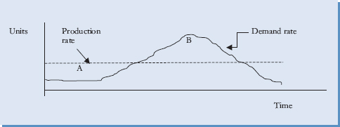
FIGURE 9.1 Differences in production and demand rates.
Another important factor are seasonal demand patterns. This may result in high and low periods of demand, such as ice cream sales in the summer or demand for snow shovels in the winter. It would be very costly for production facilities to produce products in unison with the seasonality of demand. This might mean closed facilities and unemployed workers during low seasons, and overtime production during high seasons. Switching production rates of large facilities can be extremely costly. A more common strategy is for companies, and their supply chains, to produce at a more uniform rate during the year. In this case extra products are stored in inventory and used during peak seasons. This is shown in Figure 9.1, where A represents inventory stored to be used up during segment B.
- Buffer Uncertainty. Companies know that many unexpected events may occur that impact both supply and demand. This could be a batch of damaged goods being received, an unexpected delay due to weather, or a strike at a supplier's plant. Companies carry extra inventory in stock to protect themselves or “buffer” against these uncertainties. Think about yourself going to the movies with friends. The movie ticket might cost $8.00 but you will likely carry with you a bit more money. Why? Just in case something comes up. That is the same logic.
- Economic Purchase Orders. Buying larger quantities means incurring a higher inventory holding cost. However, there are a number of reasons when this may be advantageous. For example, suppliers sometimes offer price discounts to encourage customers to purchase larger quantities at one time. Similarly, buying in large quantities may result in savings associated with transporting larger quantities at one time. Also, anticipating some type of price increase or disruption, which may lead to quantity shortages, leads companies to buy larger quantities. An example might be a drought in Africa, leading to an anticipated price increase of coffee.
TYPES OF INVENTORY
There are different types, or categories, of inventory designed to meet the different purposes for carrying inventory, and their quantities are computed differently. We look at these here.
- Cycle Stock. These are also called lot size inventories. This is inventory for immediate use and is computed based on expected demand over a certain time period. It assumes demand is known with certainty and computes how much stock is needed over a set period of time. It also accounts for the fact that products are typically produced in batches. This is the quantity, or the size, of the batch that is produced during the production cycle. Therefore it is called “cycle stock.”
- Safety Stock. Safety stock, also called buffer stock, is the extra inventory we carry to serve as a cushion for uncertainties in supply and demand. It can be in the form of finished goods to cover unexpected demand. It can also be in the form of raw materials to guard against supply problems, or in the form of WIP inventories, to guard against production stoppages.
- Anticipation inventory. As the name states, these inventories are carried in anticipation of certain events. Their one purpose is to compensate for differences in the timing of supply and demand, and to smooth out the flow of products throughout the supply chain. They are also used when demand fluctuations are significant, but predictable, such as with seasonal variation. This is where companies carry extra inventory during a low season in anticipation of higher demands during the high season. For this reason they are sometimes called seasonal inventory. Finally, these are inventories that are carried in anticipation of a price increase or a shortage of products— sometimes called hedge inventory.
- Pipeline inventory. Also called transportation inventory, this is inventory that is simply in transit. It exists because the points of demand and supply are not same. At any one time a global supply network has a large percentage of its inventory in transit—say on a barge, truck, or rail—being moved from one location to another, or waiting to be loaded or unloaded.
- Maintenance, Repair and Operating Items (MRO). In addition to inventories that directly support product creation, there are other inventories that are used indirectly. These are called maintenance, repair and operating items (MRO). They include everything from office supplies and forms, to toilet paper and cleaning supplies, to tools and parts needed to repair machines. Collectively, MRO items make up a significant amount of inventory and need to be managed like all other inventories. Consider the abundance of printing paper in an office, paper cups at Starbucks, or latex gloves in a hospital.
INVENTORY COSTS
Two of the most important inventory costs are holding cost and ordering cost. These costs typically move in opposite directions, where reducing one means increasing the other. A third important cost is shortage cost. We look at these next.
- Holding Cost. Holding cost, sometimes called carrying cost, includes all the costs that vary with the amount of inventory held in stock. This includes storage facilities, handling, insurance, pilferage, breakage, obsolescence, depreciation, taxes, and the opportunity cost of capital. Although we own the inventory, there are still costs associated with keeping it. Theft is not an uncommon occurrence; there are also damages that can occur; highly innovative or seasonal items can easily become obsolete if not sold on time.
Inventory holding cost is typically described as a percentage of the value of the inventory that is held. It is generally denoted by Hand is computed as follows:
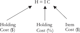
H is the dollar value to hold one unit in inventory over some period of time. I is holding cost as a percentage of item cost, and C is cost of the item. Therefore, inventory holding cost can be provided as a percentage, say 30% of cost of goods annually. It can also be provided as a dollar value, such as $12 per unit per year. Notice that holding cost must be provided over some period of time, whether a day or month or year. The longer the time period the longer we are holding inventory in stock and the higher the inventory holding cost.
Inventory holding cost is generally underestimated, and can roughly vary from 15% of cost of goods per year to as much as 50% of cost of goods. Reducing holding costs means a reduction in inventory levels and results in frequent replenishment. This, however, then results in a higher ordering cost.
- Ordering Cost. This cost includes all the costs involved in placing an order and procuring the item. It involves deciding on order quantities, clerical costs involved in placing the order, tracking the order, and receiving it. Ordering cost is sometimes called setup cost as it also includes the costs involved in preparing the production run, when the items are made in-house. If there were no costs, or loss of time, when changing from producing one product to another, companies would produce many small quantities. They would quickly switch from producing one product to another, reducing inventory levels. However, this is not the case and there is cost associated with switching production from one product type to another.
Notice that reducing ordering cost means ordering less frequently. This means that the quantities ordered have to be larger, and will result in higher levels of inventory. This lower ordering cost, unfortunately, will result in a higher inventory cost as we then have to carry more in stock. Holding and ordering costs are the most common inventory costs and the challenge is to find the right balance between them.
- Shortage costs. Shortage costs occur when we run out of stock. This cost reflects the consequences of not having enough in inventory. Being out of stock means that the customer will have to wait for the item to arrive, or the order must be cancelled. Potentially there is a loss of sale. Also, there can be loss of goodwill and reputation with customers. There is a trade-off between carrying extra stock to ensure we can satisfy demand and the costs resulting from a stock-out. This balance is sometimes difficult to obtain as it is hard to estimate true shortage cost and the impact of the shortage on customer behavior.
John Deere & Company
Excess inventory can hurt financial performance. However, companies need to have enough products in showrooms to generate sales. The trick is to maintain the bare minimum yet have enough products available to support sales. John Deere & Company had to tackle this problem in its $4 billion worldwide Commercial and Consumer Equipment (C&CE) division. The company restructured that division's supply chain to reduce inventory and freight costs. The result was a major improvement in the company's financial performance.
In 2001, the company embarked on an effort to better manage their return on assets. A large part of the assets in the C&CE division was finished goods inventory, both in the factories and in dealers' hands. In an effort to free up capital John Deere began an inventory-reduction initiative. About 70% of the finished-goods inventory was at dealers' locations, which had to be reduced. However, the dealers were uncomfortable with this decision. The reason was that many of the products sold—such as lawn mowing equipment, utility vehicles, and golf course maintenance equipment—are things that customers like to sit on, touch, and try out before finalizing their purchase. This enhances sales. Also, the seasonal nature of the sales cycle complicated the inventory-reduction effort as 65% of retail sales of lawn mowers occur between the months of March and July.
John Deere used advanced software to determine how to better align its production with demand to reduce inventory. An analysis concluded that the division could reduce inventory by $1 billion if it held the right amount at the right location at each point throughout the year. Due to concerns of dealers they chose to reduce inventory by $250 million each year over a four-year period in a process dubbed “stair-stepping.” In addition, they decided to change their supply chain processes to ensure products were available to meet demand. They would react more swiftly to changes in demand as now there was less inventory to buffer demand swings. Processes had to be changed to become faster and more flexible to support a lower inventory level.
The division began by reducing target inventory levels, which required a change in the production schedule at its five factories throughout North America. In the past these inventory targets had been set high to compensate for the inability of factories to quickly respond to changes in demand. Now production schedules had to be changed to adjust to demand. In addition, the factories changed their assembly practices, producing at a more level rather than seasonal rate.
Through this process of restructuring the supply chain, John Deere cut inventory and reduced freight costs to better manage assets and enhance shareholder value. The company learned that operating a supply chain with less inventory means adjusting internal production and distribution processes. It also means significant financial rewards.
Adapted from: James A. Cook. “Running Inventory like a Deere.” Supply Chain Quarterly, Issue 4, 2007.
INVENTORY SYSTEMS
Every inventory system must answer the two basic questions: when to order and how much to order. There are two basic categories of inventory systems that accomplish this and they work in slightly different ways. Let's look at these next.
FIXED-ORDER QUANTITY SYSTEM
The first inventory system is called a fixed-order quantity system. As the name suggests, the quantity that is ordered with this system is constant or fixed, and is denoted by Q. An order is placed when the inventory position drops to a predetermined level, noted as the reorder point or ROP. Therefore, there are two variables that define this system and answer the two basic questions of when to order and how much: Q and ROP. They specify when to place an order: when inventory reaches the reorder point ROP. They also specify how much to order: the quantity Q.
The fixed-order quantity model is shown in Figure 9.2. Notice that the system assumes a constant demand rate of d by which the inventory position (IP) is reduced. When the IP reaches the reorder point (ROP), an order is placed for the quantity Q. When goods are received the inventory is replenished and the inventory position is increased by Q. However, inventory cannot arrive the moment an order is placed as there is a certain amount of lead time, L, during which we have to wait for the order.
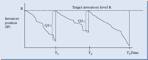
FIGURE 9.2 Fixed-order quantity system.
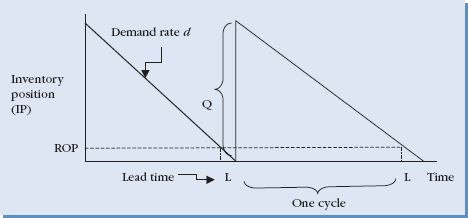
FIGURE 9.3 Fixed-time period system.
With this system inventory is checked on a continual basis and the assumption is that we always know the current level of inventory. When inventory levels reach the reorder point ROP, an order of quantity Q is placed. For example, let's assume that a hotel chain uses a fixed-order quantity system for its inventory of lavender bath soaps. Its policy is that it always orders 2,000 soaps, for which it gets a nice quantity discount, and the order is made when the number of soaps drops to 300. Therefore, the reorder point ROP = 300, and the order quantity Q = 2,000.
In the basic version of this system the order quantity Q is computed as the economic order quantity (EOQ)—an economically optimal order quantity. For this reason this system is sometimes called the EOQ model. Other terms used to describe it are the Q-model as the quantity Q is constant. Sometimes it is called a continuous review system, as the inventory levels are continuously monitored. The model has even been called a sawtooth model, as the graph of inventory looks like a sawtooth. All these terms refer to the same type of inventory system, describing different features of the system itself. Later in this chapter we will see how the EOQ value is computed.
FIXED-TIME PERIOD SYSTEM
The second inventory system is called a fixed-time period system shown in Figure 9.3. Here inventory levels are checked in fixed time periods, T, and the quantity that is ordered varies. The system sets a target inventory level, R, to be maintained. Inventory is checked every T intervals, say every week or every two weeks, and an order is placed to restore the inventory level back to R. Based on the inventory level at time period T, the amount of inventory that needs to be ordered will be some quantity Q that varies from period to period. This quantity Q is the difference between the target inventory R and how much inventory is in stock, the inventory position (IP) at time T:
Q = R − IP
- Q = order quantity
- R = target inventory level
- IP = inventory position
There are two variables that define this system and answer the two basic questions of when to order and how much are: T and Q. They specify when to place an order: at time interval T. They also specify how much to order: quantity Q, computed as the difference between the target inventory, R, and the inventory position, IP. Sometimes this system is called the Periodic Review System to indicate that the inventory level is checked periodically, rather than continuously.
Let's assume a hotel chain uses a fixed-time period model for its inventory of lavender bath soaps. Also, let's say its policy is to check inventory levels every two weeks, and that it has a target inventory level R = 5,000 soaps. If after two weeks the company checks its inventory level and finds its inventory position IP = 2,800 soaps, it would place an order for quantity Q= R – IP = 5,000 – 2,800 = 2,200 soaps.
COMPARING FIXED-ORDER QUANTITY VERSUS FIXED-TIME PERIOD SYSTEMS
Both inventory systems answer the question of when and how much to order, but they do it differently. Figure 9.4 shows a comparison of the two systems.
The biggest difference between the two systems is the timing and quantities of the orders placed. With the fixed-order quantity system inventory is checked on a continual basis and the system is prepared to place orders multiple times per year on a random basis. This has an advantage of providing greater system responsiveness, but is also requires administrative processes to be in place on a continual basis. In addition, as different inventory items may reach their reorder points at different time periods, it may be difficult to obtain quantity discounts that are based on a bundled order.
FIGURE 9.4 Comparison of inventory systems.

The fixed-period order system requires carrying more safety stock inventory. The reason is that with this system we do not check the inventory position (IP) on a regular basis and a sudden surge of demand could lead to a stock-out. This system, however, allows more organized purchasing as inventory levels are checked in set time intervals. Orders can be bundled and quantity discounts obtained easier. Imagine in our hotel example if the company used a fixed-order quantity model to place orders for various items, such as soaps, shampoos, lotions, and conditions. These different items may reach reorder points at different times generating many orders at random intervals. On the other hand, a fixed-period system could ensure that inventory levels are checked on a regular basis for all items, say every two weeks. Then the orders for all the items could be bundled.
In general, a fixed-order quantity system is more appropriate for high value items as average inventory carried is lower. Also, it is more appropriate when stock-outs are less desirable, as inventory is monitored on a continual basis. However, this system is more costly to maintain as it requires technology to record all transactions and compute the inventory position in real time.
FIXED-ORDER QUANTITY SYSTEMS
A fixed-order quantity system is one of the most important in inventory management. For that reason we need to look at how to compute the two variables that define it: the order quantity (Q) and the reorder point (ROP). Before we do that, however, we need look at the assumptions this system makes. Most importantly, the system assumes that all the variables occur at a constant rate and their values are known with certainty. For example, the system assumes that the demand, d, occurs at a constant rate and that there is no variability in demand. Also, the lead time L is constant, the holding cost His known and fixed, as are stock-out cost S and unit price C. Although these assumptions are not realistic the model is highly robust and provides excellent results despite these assumptions.
THE EOQ
The first decision in the fixed-order quantity model is to select the order quantity Q. Recall that there are a number of inventory costs, most notably inventory holding cost and ordering cost. We want to select the “best” order quantity that minimizes these costs. This is called the economic order quantity or EOQ. This is computed by looking at the total annual inventory cost and finding the order quantity that minimizes it. Consider that the total annual cost comprises annual purchase cost, annual ordering cost, and annual holding cost, and looks as follows:
Total cost = Purchase cost + Ordering cost + Holding cost

where
- TC = Total cost
- D = Annual demand
- C = Unit cost
- Q = Order quantity
- S = Ordering cost
- H = Holding cost
Let's look at these terms in a bit more detail:

The first term in the equation, DC is the annual purchase cost for items. It comprises annual demand (D) times the unit cost of each item (C). The second term ![]() S is the annual ordering cost. It is computed as the number of orders placed per year
S is the annual ordering cost. It is computed as the number of orders placed per year ![]() , times the cost of each order, S. Finally, the third term is annual holding cost where
, times the cost of each order, S. Finally, the third term is annual holding cost where ![]() is the average inventory held. Remember that our maximum inventory is Q units when the order is received. When inventory is depleted we have zero. Therefore on average we have
is the average inventory held. Remember that our maximum inventory is Q units when the order is received. When inventory is depleted we have zero. Therefore on average we have ![]() units in inventory. H is the annual holding cost per unit of inventory. Recall that H is a percentage computed as H = I C.
units in inventory. H is the annual holding cost per unit of inventory. Recall that H is a percentage computed as H = I C.
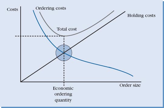
The behavior of the two costs is shown in Figure 9.5. Notice that inventory holding cost increases with the order quantity, Q. The reason is that higher order quantities mean holding more inventory. However, this also means that we are ordering less frequently so ordering cost decreases. The opposite is true as the order quantity Q is decreased. A smaller order quantity results in a lower holding cost, but a higher ordering cost, as we are ordering more frequently.
The objective is to pick an order quantity that minimizes the sum of both the holding and ordering costs, which is the minimum point on the total cost curve. This is the “best” or optimal order quantity, Qopt, also called the economic order quantity (EOQ). To find the minimum point on the total cost curve we use calculus. We take the derivative of total cost (TC) with respect to Q and set this equal to zero. For the basic model considered here, the calculations are as follows.
- Total cost equation:

- First derivative of total cost equation:

- Solving the above equation for Q we compute Q opt, also called the EOQ:

This is the EOQ or the “best” quantity to order in the fixed-order quantity system in order to minimize the sum of inventory cost and ordering cost.
Example Computing the EOQ at Georgia's Florists
You have taken over as inventory manager at Georgia's Florists. You would like to use EOQ to compute the best quantity of orchids to order. The previous manager at Georgia's ordered orchids once a month in quantities of 1,000 to simply match the monthly demand. Orchids are expensive to order with an ordering cost of $300 per order. Holding cost is estimated at 15% of product cost annually, with a product cost of $60 per unit.
What would be your order? What is the number of orders per year? What is the annual holding cost? Assuming four weeks/month and a lead time of one week, what is the reorder point?
Answer: You were given the following information:
Annual demand (D) = 1,000 orchids per month × 12 months = 12,000 orchids
Holding cost (H) = (.15)60 per unit
Ordering cost (S) = $300 per order
Computing the EOQ:

REORDER POINT (ROP)
The EOQ answers the question of how much to order, but we still need to determine when to order. Assume that the demand rate, d, and lead time (L) are constant and known with certainty. In that case the reorder point would simply be enough inventory to ensure that demand is covered during the length of the lead time. In this simple case, the reorder point would be computed as:
ROP = demand during lead time
ROP = d L
Let's go back to the Georgia Florists example. If lead time L is one week and the demand, d, is 250 units per week the ROP would be:
Reorder Point = ROP = d × L = 1 week × 250 = 250 units
The order policy for Georgia's Florists would be defined by the EOQ and ROP. This would mean ordering 895 orchids when inventory drops to 250 orchids.
SAFETY STOCK
Unfortunately, d and L are rarely fixed, and demand is often higher than expected. As a result we have to carry a bit more inventory to address this uncertainty. This is called safety stock or buffer stock, and is inventory we carry in addition to the demand during lead time. Safety stock is added to the ROP calculation and is computed as follows:
ROP = demand during lead time + safety stock
ROP = d L + SS
ROP = d L + ZkσL
We can see that SS is equal to Zk σ L. Let's look at this second term in the equation to see what it means. Zk is the value of the standard normal variable for a particular service level k. The service level, k, is simply the probability that we will not run out of stock. This is set by the company based on the level of service they wish to provide for a particular product and customer base. Higher service levels mean higher levels of inventory. For example, a service level k of 95% means a 95% probability of being in stock and a 5% probability (100% – 95%) of being out of stock. The value of Z is obtained from the standard normal table in the back of the text for a particular value of k.
The service level, k, can be set in two ways:
- Directly. This is a specified percentage, such as 95% service level.
- Indirectly. This may be in terms of the number of stock-outs tolerated, such as five stock-outs per year. If we know the number of orders per year we can then compute the value of k.
The second part of this term, σ L, is standard deviation of demand over the lead time L. The higher the variability the higher the standard deviation (computed as the square root of variance), the higher the safety stock.
Example Computing Safety Stock at Georgia's Florists
Earlier we computed an EOQ and ROP for Georgia's Florists, but assumed no safety stock. Let's now compute the amount of safety stock and the new ROP, assuming that you desire a 95% service level.
Answer: We know the following:
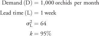

Therefore, the new order policy would be to order 895 orchids when inventory drops to 263 orchids.
ECONOMIC PRODUCTION QUANTITY (EPQ)
The fixed-order quantity model assumes that the EOQ arrives in one lump sum after the order is placed. In the Georgia's Florists example, all the ordered orchids arrived in one shipment. This meant that the company had to have physical space for the entire EOQ quantity. Sometimes, however, the products ordered are made in-house or in close proximity. In that case the producing operation may not wait to produce all Q units before passing them on to the operation that ordered them. This is called the economics production quantity (EPQ) and sometimes it is called the production rate model. The variables that define this model are still Q and ROP, as these define how much to order and when. However, the computation of Q is a little bit different.
Consider Samba Chocolate Co. that produces a variety of chocolates and makes their own packaging for their specialty chocolate: turtle truffles. The turtle truffle wrapping is made immediately next door to chocolate production. The chocolate production department orders the special wrapping from the packaging department. However, the packaging department does not wait to make all Q units of wrapping before they get it to chocolate production. Rather, they begin passing the wrapping to chocolate production as it is being produced. If the wrapping is made at a rate of 80 units per day and chocolate production uses it at a rate of 60 units per day, the inventory will build up at a rate of 20 units per day. This is shown in Figure 9.6.
Figure 9.7 illustrates the way the EPQ system works. As with the basic fixed-order quantity model a quantity Q is ordered at the ROP. The production process starts at a rate of p. However, as the product is produced it is used at a rate of d, with d ≤ p, and inventory builds up at rate of p – d. Production stops once the ordered quantity Q has been made. This is one cycle. The cycle beings again when the ROP is reached.
FIGURE 9.6 Production and demand at Samba Chocolate Co.
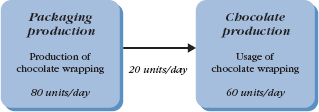
FIGURE 9.7 Economic production quantity system.
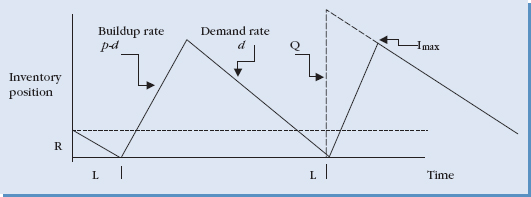
Notice that with this system we hold less inventory than with the basic EOQ system. The reason is that here we are using part of the inventory while it is being produced. The broken line in Figure 9.7 shows the amount of inventory Q that we would hold if the inventory was received all at once. Instead, the maximum amount of inventory that we hold—Imax—is shown as the inventory peak.
The optimal quantity that should be ordered in this situation is different from the traditional EOQ as the inventory holding cost is lower. As before, to compute the optimal order quantity Q opt we begin with the total cost equation:
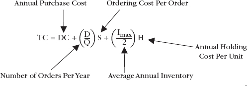
Notice that in this equation the average annual inventory is computed as ![]() rather than
rather than ![]() as in the basic EOQ derivation. The reason is that the maximum inventory we hold is no longer Q, but is Imax.
as in the basic EOQ derivation. The reason is that the maximum inventory we hold is no longer Q, but is Imax.
To compute the Q opt consider the following. Time to produce Q units is ![]() During this time we lose to demand d
During this time we lose to demand d ![]() units. Therefore, the maximum held in inventory, Imax, computed as:
units. Therefore, the maximum held in inventory, Imax, computed as:
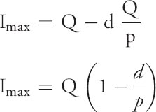
d = daily demand rate
p = daily production rate
Substituting this into the total cost equation we get the following:

Using calculus we solve for Q obtaining the equation for Q opt:

Example Calculating EPQ and Imax
A bicycle manufacturer uses 50,000 wheels per year for its popular children's cycle. The firm makes its own wheels, which it can produce at a rate of 600 per day. The bicycles are assembled uniformly over the entire year. Carrying cost is $1 per wheel a year, and setup cost for a production run of wheels is $45. Considering that the plant operates 250 days per year, find the order quantity and Imax.
Solution: The order quantity here is the EPQ. We just need to substitute values provided into the equation as follows.

Be careful when substituting to make sure that the units of time are the same in each denominator. Demand is given to be 50,000 wheels per year, which we use in the first denominator as holding cost H is also given per year. However, the production rate p is given per day and we must convert demand to a daily rate here.

Although the order is 2,598 wheels, there only needs to be space for 1,732 wheels.
FIXED-TIME PERIOD SYSTEMS
In a fixed-time period system, inventory levels are checked in regularly set time intervals. The goal is to place an order to restore the inventory position to the target inventory level R. Therefore, the quantity that is ordered at time interval T is:
Q = R − IP
where
- Q = order quantity
- R = target inventory level
- IP = inventory position at time T
In this system the questions of when to order and how much are set as follows. Orders are placed at time interval T. This time interval is typically set for organizational convenience. For example, it may be every week, every two weeks, or once a month. The ordering process requires administrative responsibility and the organization decides what is most convenient. Also, sometimes suppliers make routine visits to customers and this timing may be considered when setting T. Finally T can even be set as the time interval that would allow for a certain quantity Q to be used up. This could be, for example, the optimal order quantity EOQ:

The quantity Q that is ordered is the amount that will restore inventory levels back to R, the target inventory level. Therefore, the important decision is computing the target inventory level.
COMPUTING TARGET INVENTORY
The target inventory level needs to be large enough to cover three types of demand:
- Demand during the length of the lead time L.
- Demand during the length of the review period T.
- Safety stock, SS, to guard against uncertainty.
Therefore, the target inventory level can be computed as follows:
R = demand during lead time + demand during review period + safety stock
R = dL +d T+ ZkσL+T
As before, Zk is the standard normal variable for the desired service level. However, standard deviation of demand is now over both the length of the lead time L and the review period T. Sometimes the standard deviation is provided over another time period t, other than the specified L + T. It is easy to make a mathematical conversation using the following equation:

where
- t = interval over which standard deviation is given
- L = lead time
- T = review interval
Notice that the demand, lead time, and review period are over length of time, such as days, weeks, or years. Remember, however, that this length must be the same throughout the equation.
Example Computation of the Fixed-Time Period System
Gordon's Potato Chips reviews inventory every 14 days, with demand and lead time given below:
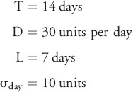
If the company tolerates no more than two stock-outs per year, develop the ordering policy for a fixed-time period inventory system.
Solution: Remember that an ordering policy specifies when to order and how much. Here we know that orders are placed every 14 days. To determine how much to order we must first compute the target inventory level R and substitute known values:

Notice that we still have to compute k, the cycle service level. Let's look at what we know:
- two stockouts per year
- an order placed every two weeks
- 52 weeks/year means 26 orders per year (52/2)
Therefore, the service level
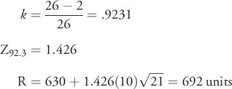
Therefore, the ordering policy is to check inventory every two weeks and order the quantity that will restore inventory to 692 units.
INDEPENDENT VERSUS DEPENDENT DEMAND
One of the biggest differences in inventory is between dependent and independent demand. Understanding this difference is important as the entire inventory policy for an item is based on this. Independent demand is demand for a finished product, such as a computer, a bicycle, or a pizza. Dependent demand, on the other hand, is demand for component parts or subassemblies. For example, this would be the microchips in the computer, the wheels on the bicycle, or the amount of cheese on the pizza.
The inventory systems we discussed thus far are for independent demand. Dependent demand is derived from its independent demand. We can forecast the amount of bicycles we expect to sell, then we can derive the quantities needed of wheels, tires, frame, and other component parts. For example, if a company plans to produce 200 bicycles in a day, it would need 400 wheels, 400 tires, and 200 frames.
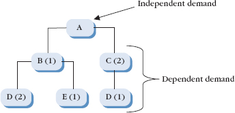
FIGURE 9.8 A simple bill of materials (BOM).
The number of wheels, tires, frame, and other component parts is dependent upon the quantity of the independent demand item from which it is derived.
The relationship between independent and dependent demand is shown in a bill of materials (BOM), which can be in the form of a table or a visual diagram. An example is shown in Figure 9.8. Item A is the independent demand item. All the other items are dependent demand. The quantities that go into the final item are shown in parentheses. Notice that two units of C are combined with one unit of B to make the final product. Similarly, two units of D and one unit of E are combined to make one unit of B.
Dependent demand order quantities are computed using a system called material requirements planning (MRP), which considers not only the quantities of each of the component parts needed, but also the lead times needed to produce and receive the items. For example, 20 units of A means that 20 units of B are needed, as are 40 units of C. Similarly, 40 units of D and 20 units of E. However, the system must also take into account differences in lead times, as receiving D may have a different lead time than receiving E. This means that the orders should be placed at different times. This system can also be tied to costs of goods, and can link internal and external members of the supply chain. This is called enterprise resource planning (ERP), discussed in Chapter 3.
Intel Corporation
Companies that make component parts are highly dependent on the success of the final product— their independent demand item. An example of this is Intel Corporation that has become famous for their microprocessors, or chips, that run PCs. The problem for Intel has been the declining PC market, signaling a decline in demand for their chips and the famous “Intel inside” logo.
To leverage its dependent demand position, Intel has come up with a new strategy. It has created a new kind of chip—the Atom chip—that can act as the brains of a variety of electronic devices rather than just computers or mobile phones. Two years ago, Intel even held a contest for college students, asking them to come up with new uses for the company's Atom processor. One proposal was a shower that regulates water temperature and plays music from the Internet. While Intel doesn't plan to enter the shower market, it is putting its chips into gas pumps, cars, musical instruments, and other devices, where few processors have gone before. The company understands that there is a limit to where their core business will take them. They understand that their growth depends on sales of their independent demand items, and are counting on the new chip to break their dependence on the slowing PC market. By expanding their independent demand options they are growing their own sales.
Adapted from: “Intel Wants to Be Inside Everything,” Bloomberg Businessweek, September 6–12, 2010.
MANAGING SUPPLY CHAIN INVENTORY
The quantitative models we discussed help managers determine when and how much to order. However, managers should not just follow the models blindly. There are a number of practical implications to consider when managing supply chain inventories. We discuss these here.
ABC INVENTORY CLASSIFICATION
All items in the supply chain are not of equal importance. Some are very important, such as specialized surgical equipment. Others are less important, such as latex gloves in a hospital. The first step in managing inventory is to classify inventory based on its degree of importance in order to manage it properly. The tool for this is ABC classification. Classifying inventory based on degree of importance allows us to give priority to important inventory items and manage those with care. It also prevents us from wasting precious resources on managing items that are of less importance.
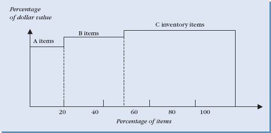
ABC classification is based on Pareto's Law, which states that a small percentage of items account for a large percentage of value. This value can be sales, profits, or other measure of importance. Roughly 10% to 20% of inventory items account for 70% to 80% of inventory value. These highly valuable items are classified as A inventory items. Moderate value items account for approximately 30% of inventory items and contribute to roughly 35% of the total. They are called B items. Finally, approximately 50% of the items only contribute to roughly 10 percent of total inventory value. These are called C items and are of least importance. Figure 9.9 provides an example of ABC analysis.
Conducting an ABC classification of inventory is quite easy. The steps are as follows:
- Determine annual usage or sales for each item.
- Determine the percentage of the total usage or sales by item.
- Rank the items from highest to lowest percentage.
- Classify the items into groups.
After ranking the items from highest to lowest percentage, do not force groups to fit the preset percentages, as these are rough estimates. Rather, there are typically natural breaking points that will occur. The data will naturally group itself and these are groupings that should be used.
FIGURE 9.9 ABC classification of inventory.
ABC analysis is extremely important for determining order policies. The most sophisticated inventory systems should be used for A items. In fact, many managers personally oversee these. By contrast, C items are typically left for automated ordering systems as they do not warrant the cost of managerial involvement.
ABC analysis is also important in establishing safety stock levels. Remember that safety stock is extra inventory held to guard against uncertainty of demand and prevent stock-outs. All inventory items are not of equal importance and the safety stock policy will be different based on ABC classification. The importance of not running out of stock of a particular item will enter the safety stock computation through the service level component, k. For example, a service level of 80% results in a significantly lower safety stock than a 98% service level. ABC classification is a critical part of the stocking decision given the costs of holding extra inventory, as well as the costs of stocking out.
PRACTICAL CONSIDERATIONS OF EOQ
There are a number of practical considerations that must be considered when using the EOQ, rather than applying it blindly.
- Lumpy Demand (POQ). EOQ assumes demand to be uniform. However, product demand can sometimes be “lumpy.” This means that it occurs in a discontinuous or nonuniform fashion, with some periods exhibiting high demand and then other periods having zero demand. Using EOQ in this case results in carrying too much inventory over periods with no demand. A more practical option here is to use something called a periodic order quantity (POQ).
As with EOQ, the logic behind the POQ is to balance ordering and holding costs. The difference, however, is that ordering is done in whole periods of demand. To determine the number of periods to order, the first step is to compute the EOQ quantity. Next, we determine the average number of periods of demand covered by the EOQ, and then order that quantity rounding up. For example, let's say that weekly demand is 120 units with an EOQ of 350 units. This means the EOQ covers an average of 350/120 = 2.9 weeks of demand. This rounds to an “economic order period” of three weeks, meaning that we always order three weeks of demand at a time. This is the POQ.
- EOQ Adjustments. Recall that the EOQ was computed as the minimum point on the total cost curve. However, this total cost curve is pretty flat around the minimum point. It is a soft curve rather than a sharp minimum point. This means that ordering slightly above or below the minimum point does not substantially change the total cost. This allows managers to increase or decrease the EOQ—within reason, of course—to accommodate container sizes, truck loads, and various types of discounts.
- Capacity Constraints. When computing anticipation inventory we typically consider the balance between inventory holding cost and anticipated costs we are trying to avoid. One additional factor that needs to be considered is capacity or storage size. Ordering extra inventories to hedge against a price increase may result in unanticipated expenses if additional storage space needs to be leased.
MEASURING INVENTORY PERFORMANCE
Inventory impacts the supply chain both in terms of customer service and cost. Given its importance, success of inventory policy must be measured and evaluated on a regular basis. The most common metrics to measure inventory are:
- Units
- Dollars
- Weeks of Supply
- Inventory Turns
The first two measures directly address the number of units available and the dollars tied up in inventory. The last two measures were discussed in Chapter 7. Recall that “weeks of supply” is a measure of inventory quantity relative to usage and “inventory turnover” gives us a sense of inventory movement. Their computations are as follows:

In Chapter 7 we were given average inventory value. Now that we know a bit about ordering policy we can compute it as follows:

The inventory turnover for an individual item is then computed as:

Example Average Inventory Calculation
Suppose that an item is being managed using a fixed-order quantity model with safety stock. The following information is given:
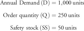
What are the average inventory and inventory turn for the item?
Solution:

VENDOR MANAGED INVENTORY (VMI)
Historically companies owned and managed all of their inventories. They were responsible for the storing, controlling, replenishing, and overall management of the inventory. With SCM, most of this has changed. Today, many firms have implemented vendor managed inventory (VMI) arrangements. Here, the vendor is responsible for managing the inventory located at a customer's facility. The vendor stocks the inventory, places replenishment orders, and arranges its display. The vendor typically own the inventory until it is purchased by the customer.
VMI offers a number of important advantages to both the customer and the vendor. The vendor has greater control over their product. They are required to work much more closely with the customer, giving them better understanding of how to serve the market. The customer, in turn, has less responsibility and financial burden over the inventory items. VMI requires both the vendor and customer to work closely together. It represents one of the many partnership arrangements that have evolved in supply chain management.
CHAPTER HIGHLIGHTS
- There are many reasons for carrying inventory. They include protecting against lead time demand, maintaining independence of operations, balancing supply and demand, buffering against uncertainty, and achieving economic purchase orders.
- There are different types of inventory intended for different purposes. Inventory types are: cycle stock, safety stock, anticipation inventory, pipeline inventory, and MRO.
- The three inventory costs are: holding cost, ordering cost, and shortage cost. Inventory holding cost includes all the costs involved with holding inventory in stock. Ordering cost is the cost of placing an order. Shortage cost is the cost associated with being out of stock, such as loss of customer goodwill and possible lost sales.
- Inventory systems answer two basic questions: when to order and how much to order. Two of the most common types of inventory systems are: fixed-order quantity system and fixed-time period system.
- In a fixed-order quantity system the order placed is constant or fixed. An order is placed when the inventory position drops to the reorder point, noted as ROP. In the basic fixed-order quantity system the order quantity is computed as an economic order quantity or EOQ. When production directly feeds demand, then it is computed as an economic production quantity or EPQ.
- In a fixed-time period system orders are placed in regular time intervals denoted by T. The order that is placed varies and is the quantity that will return the IP to a target inventory level, denoted as R.
- Independent demand is demand for a finished product, such as a computer, a bicycle, or a pizza. Dependent demand is demand for component parts or subassemblies that are a result of the independent demand item.
- To manage inventory properly it must be classified based on its degree of importance. The tool for this is ABC classification. This allows us to give priority to important inventory items and manage those with care, while not wasting resources on items that are of less importance. A inventory items are of highest importance and must be monitored carefully. B items are classified as moderate importance, and C items are of least importance.
- Inventory must be measured and evaluated on a regular basis given its impact on cost and customer service. The most common ways to measure inventory are in units, dollars, weeks of supply, and inventory turns.
- Vendor managed inventory (VMI) is an arrangement where the vendor is responsible for managing the inventory located at a customer's facility. The vendor stocks the inventory, places replenishment orders, and arranges its display. The vendor typically own the inventory until it is purchased by the customer.
KEY TERMS
- Inventory policy
- Buffer stock
- Seasonal inventory
- Hedge inventory
- Transportation inventory
- Holding cost
- Ordering cost
- Shortage cost
- Carrying cost
- Dollar value
- Percentage of item cost
- Setup cost
- Fixed-order quantity system
- Bill of materials (BOM)
- Material requirements planning (MRP)
- Enterprise resource planning (ERP)
DISCUSSION QUESTIONS
- Identify an example of inventory in your own life. Estimate how much it costs you to hold this inventory. Estimate the “ordering cost.” How often do you replenish this inventory and which of the inventory policies does this most closely resemble?
- Think of a service you recently used. How might this service be restructured to create service inventory as in the example of Zoots? What would they have to do? What advantages would the company gain and how would they better serve their customers?
- Find at least one business example of a fixed-order quantity system versus a fixed-period quantity system. What are their differences? Which do you think is better and why?
- Provide an example of ABC classification in a business you are familiar with. What would be the A inventory items versus B and C? What ordering policies would you use for each of these?
- Identify an example of VMI. Explain the benefits to both the vendor and retailer. Identify some of the risks for both parties.
PROBLEMS
- Ricky Orange's annual demand is 12,500 units. Ordering cost is $100 per order. Holding cost is estimated at 20% of product cost which is $50 per unit. What is the number of orders per year using EOQ to compute the best quantity to order? What is the annual holding cost? What is the reorder point? Assume four weeks/month, lead time L is one week and demand rate is 250 units per week.
- You are inventory manager of Diego Supplies Inc. You computed the EOQ to be 500 units. Annual demand for the company is 5,000 units and holding cost is $4 per unit. What is the ordering cost?
- G-Tech's monthly demand is 250 units. You are in charge of the inventory department. You know that the holding cost is $60 per unit and ordering cost is $100 per order. What is the EOQ? What is the number of orders per year? What is the annual holding cost? If lead time L is one week and demand rate is 60 units per week, what is the ROP?
- We know that Blue Pad Company's lead time L is one week and demand rate is 100 units per week. Compute the amount of Safety Stock and new ROP assuming that the company desires a 98% service level. Standard deviation of demand over lead time is eight.
- Bright Light computed their new ROP to be 116.45. Assume that lead time L is one week and demand rate is 100 units per week. What is the company's desired service level assuming standard deviation of demand over lead time is 10?
- Basic Code Tech desires a 95% service level to compute their safety stock. Variance of demand over lead time is 64. We computed its new ROP to be 14.16. What is the demand rate per week if we assume its lead time L is one week?
- The Yacht Company builds personal yachts. Its annual demand is 10 yachts. This company can build at a rate of one yacht per month. Carrying cost is very expensive and is about $10,000 per year. The setup cost for a production run of yachts is $2,000. Find the order quantity and I max.
- Linden Jet's annual demand is 20. It can build at a rate of four jets per month. The setup cost for a production run of jets is $1,000. Find the order quantity and I max assuming carrying cost is $1,000 per year.
- Lugini Watch's annual demand is 100. It can produce at a rate of 10 watches per month with a $100 setup cost for the production run. Find the order quantity and I max assuming carrying cost is $100 per unit.
- Apple Cakes reviews inventory every two weeks with lead time of seven days, demand rate 40 units per day and standard deviation five units per day. If the company tolerates no more than one stock-out per year, develop the ordering policy for a fixed-time period inventory system assuming 52 weeks per year.
- Ice Ginger reviews inventory every two weeks. As the inventory manager of the company, you know that its lead time is seven days and its demand rate is 40 units per day. Given variance is 25 units per day, you calculated the target inventory level to be 881 units. Now, how many stock-outs per year are permitted by the company assuming 52 weeks per year? Show all calculations.
- Pure Grapes reviews inventory every week. Lead time L is seven days and demand rate is 100 units per day. You know the company's standard deviation is 10 units per day and allows one stock-out per year. Develop the ordering policy for a fixed-time period inventory system assuming 52 weeks per year and 95% service level.
REFERENCES
Callioni, Gianpaolo, Xavier de Montgros, Regine Slagmulder, Luk N. Van Wassenhove, and Linda Wright. “Inventory Driven Costs.” Harvard Business Review, March 2005: 135–141
Green, James H. Production and Inventory Control Handbook, 3rd edition. New York: McGraw-Hill, 1997.
Lee, H. L. “Aligning Supply Chain Stratgies with Product Uncertainties.” California Management Review. 44(3), Spring 2002: 105–119
Silver, Edward E., David F. Pyke, and Rein Peterson. Inventory Management, Production Planning, and Scheduling, 3rd edition. New York: John Wiley & Sons, 1998.
Tersin, Richard J. Principles of Inventory and Materials Management, 4th edition. Upper Saddle River, NJ: Prentice Hall, 1994.
Timme, Stephen G. and Christine Williams-Timme. “The Real Cost of Holding.” Supply Chain Management Review. July/August 2003: 30–37.

