An emerging area for applying is the stock market trading, where a trader acts like a reinforcement agent since buying and selling (that is, action) particular stock changes the state of the trader by generating profit or loss, that is, reward. The following figure shows some of the most active stocks on July 15, 2017 (for an example):

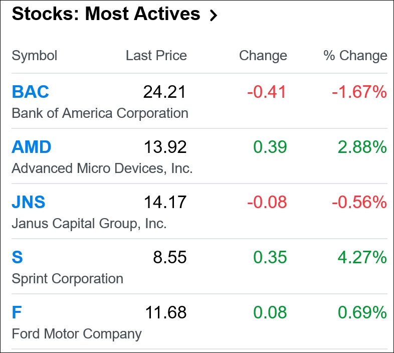
Figure 6: https://finance.yahoo.com/

Now, we want to develop an intelligent agent that will predict stock prices such that a trader will buy at a low price and sell at a high price. However, this type of prediction is not so easy and is dependent on several parameters such as the current number of stocks, recent historical prices, and most importantly, on the available budget to be invested for buying and selling.

The states in this situation are a vector containing information about the current budget, current number of stocks, and a recent history of stock prices (the last 200 stock prices). So each state is a 202-dimensional vector. For simplicity, there are only three actions to be performed by a stock market agent: buy, sell, and hold.

So, we have the state and action, what else do you need? Policy, right? Yes, we should have a good policy, so based on that an action will be performed in a state. A simple policy can consist of the following rules:

To find the stock prices, we can use the yahoo_finance library in Python. A general warning you might experience is "HTTPError: HTTP Error 400: Bad Request". But keep trying.

Now, let's try to get familiar with this module:

>>> from yahoo_finance import Share
>>> msoft = Share('MSFT')
>>> print(msoft.get_open())
72.24=
>>> print(msoft.get_price())
72.78
>>> print(msoft.get_trade_datetime())
2017-07-14 20:00:00 UTC+0000
>>>

So as of July 14, 2017, the stock price of Microsoft Inc. went higher, from 72.24 to 72.78, which means about a 7.5% increase. However, this small and just one-day data doesn't give us any significant information. But, at least we got to know the present state for this particular stock or instrument.

To install yahoo_finance, issue the following command:

$ sudo pip3 install yahoo_finance 

Now it would be worth looking at the historical data. The following function helps us get the historical data for Microsoft Inc:

def get_prices(share_symbol, start_date, end_date, cache_filename):
    try:
        stock_prices = np.load(cache_filename)
    except IOError:
        share = Share(share_symbol)
        stock_hist = share.get_historical(start_date, end_date)
        stock_prices = [stock_price['Open'] for stock_price in stock_hist]
        np.save(cache_filename, stock_prices)
    return stock_prices

The get_prices() method takes several parameters such as the share symbol of an instrument in the stock market, the opening date, and the end date. You will also like to specify and cache the historical data to avoid repeated downloading. Once you have downloaded the data, it's time to plot the data to get some insights.

The following function helps us to plot the price:

def plot_prices(prices):
    plt.title('Opening stock prices')
    plt.xlabel('day')
    plt.ylabel('price ($)')
    plt.plot(prices)
    plt.savefig('prices.png')

Now we can call these two functions by specifying a real argument as follows:

if __name__ == '__main__':
    prices = get_prices('MSFT', '2000-07-01', '2017-07-01', 'historical_stock_prices.npy')
    plot_prices(prices)

Here I have chosen a wide range for the historical data of 17 years to get a better insight. Now, let's take a look at the output of this data:

Figure 7: Historical stock price data of Microsoft Inc. from 2000 to 2017

The goal is to learn a policy that gains the maximum net worth from trading in the stock market. So what will a trading agent be achieving in the end? Figure 8 gives you some clue:

Figure 8: Some insight and a clue that shows, based on the current price, up to $160 profit can be made

Well, figure 8 shows that if the agent buys a certain instrument with price $20 and sells at a peak price say at $180, it will be able to make $160 reward, that is, profit.

So, implementing such an intelligent agent using RL algorithms is a cool idea?

From the previous example, we have seen that for a successful RL agent, we need two operations well defined, which are as follows:

To be more specific, given a state, the decision policy will calculate the next action to take. On the other hand, improve Q-function from a new experience of taking an action.

Also, most reinforcement learning algorithms boil down to just three main steps: infer, perform, and learn. During the first step, the algorithm selects the best action (a) given a state (s) using the knowledge it has so far. Next, it performs the action to find out the reward (r) as well as the next state (s').

Then, it improves its understanding of the world using the newly acquired knowledge (s, r, a, s') as shown in the following figure:

Figure 9: Steps to be performed for implementing an intelligent stock price prediction agent

Now, let's start implementing the decision policy based on which action will be taken for buying, selling, or holding a stock item. Again, we will do it an incremental way. At first, we will create a random decision policy and evaluate the agent's performance.

But before that, let's create an abstract class so that we can implement it accordingly:

class DecisionPolicy:
    def select_action(self, current_state, step):
        pass
    def update_q(self, state, action, reward, next_state):
        pass

The next task that can be performed is to inherit from this superclass to implement a random decision policy:

class RandomDecisionPolicy(DecisionPolicy):
    def __init__(self, actions):
        self.actions = actions
    def select_action(self, current_state, step):
        action = self.actions[random.randint(0, len(self.actions) - 1)]
        return action

The previous class did nothing except defining a function named select_action (), which will randomly pick an action without even looking at the state.

Now, if you would like to use this policy, you can run it on the real-world stock price data. This function takes care of exploration and exploitation at each interval of time, as shown in the following figure that form states S1, S2, and S3. The policy suggests an action to be taken, which we may either choose to exploit or otherwise randomly explore another action. As we get rewards for performing an action, we can update the policy function over time:

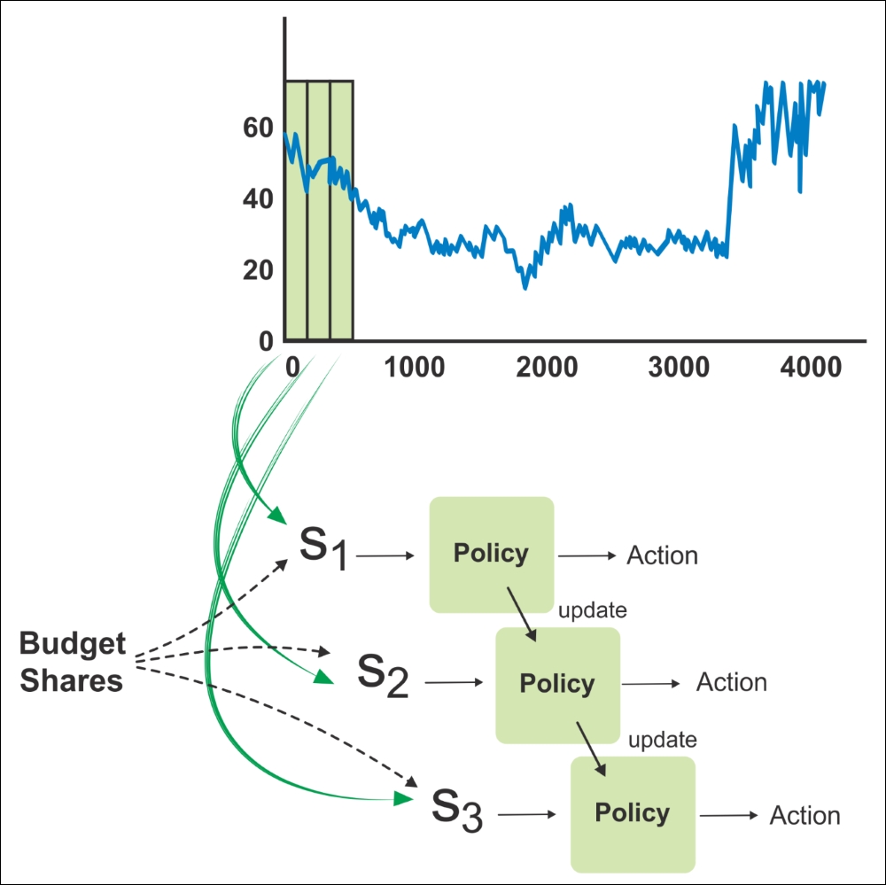
Figure 10: A rolling window of some size iterates through the stock prices over time

Fantastic, so we have the policy and now it's time to utilize this policy to make decisions and return the performance. Now, imagine a real scenario—suppose you're trading on Forex or ForTrade platform, then you can recall that you also need to compute the portfolio and the current profit or loss, that is, reward. Typically, these can be calculated as follows:

portfolio = budget + number of stocks * share value
reward = new_portfolio - current_portfolio

At first, we can initialize values that depend on computing the net worth of a portfolio, where the state is a hist+2dimensional vector. In our case, it would be 202 dimensional. Then we define the range of tuning the range up to:

Length of the prices selected by the user query – (history + 1), since we start from 0, we subtract 1 instead. Then, we should calculate the updated value of the portfolio and from the portfolio, we can calculate the value of the reward, that is, profit.

Also, we have already defined our random policy, so we can then select an action from the current policy. Then, we repeatedly update the portfolio values based on the action in each iteration and the new portfolio value after taking the action can be calculated. Then, we need to compute the reward from taking an action at a state. Nevertheless, we also need to update the policy after experiencing a new action. Finally, we compute the final portfolio worth:

def run_simulation(policy, initial_budget, initial_num_stocks, prices, hist, debug=False):
    budget = initial_budget
    num_stocks = initial_num_stocks
    share_value = 0
    transitions = list()
    for i in range(len(prices) - hist - 1):
        if i % 100 == 0:
            print('progress {:.2f}%'.format(float(100*i) / (len(prices) - hist - 1)))
        current_state = np.asmatrix(np.hstack((prices[i:i+hist], budget, num_stocks)))
        current_portfolio = budget + num_stocks * share_value
        action = policy.select_action(current_state, i)
        share_value = float(prices[i + hist + 1])
        if action == 'Buy' and budget >= share_value:
            budget -= share_value
            num_stocks += 1
        elif action == 'Sell' and num_stocks > 0:
            budget += share_value
            num_stocks -= 1
        else:
            action = 'Hold'
        new_portfolio = budget + num_stocks * share_value
        reward = new_portfolio - current_portfolio
        next_state = np.asmatrix(np.hstack((prices[i+1:i+hist+1], budget, num_stocks)))
        transitions.append((current_state, action, reward, next_state))
        policy.update_q(current_state, action, reward, next_state)
    portfolio = budget + num_stocks * share_value
    if debug:
        print('${}	{} shares'.format(budget, num_stocks))
    return portfolio

The previous simulation predicts a somewhat good result; however, it produces random results too often. Thus, to obtain a more robust measurement of success, let's run the simulation a couple of times and average the results. Doing so may take a while to complete, say 100 times, but the results will be more reliable:

def run_simulations(policy, budget, num_stocks, prices, hist):
    num_tries = 100
    final_portfolios = list()
    for i in range(num_tries):
        final_portfolio = run_simulation(policy, budget, num_stocks, prices, hist)
        final_portfolios.append(final_portfolio)
    avg, std = np.mean(final_portfolios), np.std(final_portfolios)
    return avg, std

The previous function computes the average portfolio and the standard deviation by iterating the previous simulation function 100 times. Now, it's time to evaluate the previous agent. As already stated, there will be three possible actions to be taken by the stock trading agent such as buy, sell, and hold. We have a state vector of 202 dimension and budget only $1000. Then, the evaluation goes as follows:

actions = ['Buy', 'Sell', 'Hold']
    hist = 200
    policy = RandomDecisionPolicy(actions)
    budget = 1000.0
    num_stocks = 0
    avg,std=run_simulations(policy,budget,num_stocks,prices, hist)
    print(avg, std)
>>>
1512.87102405 682.427384814

The first one is the mean and the second one is the standard deviation of the final portfolio. So, our stock prediction agent predicts that as a trader you/we could make a profit about $513. Not bad. However, the problem is that since we have utilized a random decision policy, the result is not so reliable. To be more specific, the second execution will definitely produce a different result:

>>> 
1518.12039077 603.15350649 

Therefore, we should develop a more robust decision policy. Here comes the use of neural network-based QLearning for decision policy. Next, we will see a new hyperparameter epsilon to keep the solution from getting stuck when applying the same action over and over. The lesser its value, the more often it will randomly explore new actions:

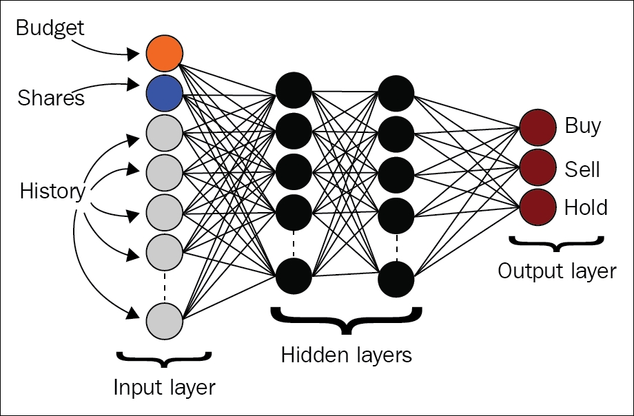
Figure 11: The input is the state space vector with three outputs, one for each output's Q-value

Next, I am going to write a class containing their functions:

Refer to the following code:

        action_q_vals = np.squeeze(np.asarray(action_q_vals))
        self.sess.run(self.train_op, feed_dict={self.x: state, self.y: action_q_vals})