With feedforward neural networks, we achieved good training performance with MNIST and Fashion-MNIST datasets. But images in these datasets are simple and centered within the input space that contains them. That is, they are centered within the pixel matrix that holds them. Input space is all the possible inputs to a model.
Feedforward neural networks are very good at identifying patterns. So, if images occupy the same position within their input space, feedforward nets can quickly and effectively identify image patterns. And, if images are simple in terms of number of image pixels, patterns emerge more easily. But, if images don’t occupy the same positions in their input spaces, feedforward nets have great difficulty identifying patterns and thereby perform horribly! So we need a different model to work with these types of images.
We can train complex and off-center images with convolutional neural networks and get good results. A convolutional neural network (CNN or ConvNet) is a class of deep neural networks most commonly applied to visual imagery analysis. CNNs are inspired by their resemblance to biological processes in that the connectivity between neurons resembles the organization of the visual cortex in humans.
A CNN works differently than a feedforward network because it treats data as spatial. Instead of neurons being connected to every neuron in the previous layer, they are instead only connected to neurons close to them, and all have the same weight. The simplification in the connections means that the network upholds the spatial aspect of the dataset.
Suppose the image is a profile of a child’s face. A CNN doesn’t think the child’s eye is repeated all over the image. It can efficiently locate the child’s eye in the image because of the filtering process it undertakes.
A CNN processes an image dataset by assigning importance to various elements in each image, which enables it to differentiate between images. Importance is calibrated with learnable weights and biases. Preprocessing is much lower when compared to other classification algorithms because a CNN has the ability to learn how to adjust its filters during training.
The core building block of a CNN is the convolutional layer. A convolutional layer contains a series of filters that transform an input image by extracting features into feature maps for consumption by the next layer in the network. The transformation convolves the image with a set of learnable filters (or convolutional kernels) that have a small receptive field.
Convolution preserves the relationship between pixels by learning image features using small squares of input data. A convolutional kernel is a filter used on a subset of the pixel values of an input image. So a convolutional kernel is one of the small squares of input data that learns image features. A receptive field is the part of an image where a convolutional kernel operates at a given point in time. Feature maps of a CNN capture the result of applying convolutional kernels to an input image. So individual neurons respond to stimuli only in a restricted region of the receptive field (or visual field).
Whew! Simply, a convolutional kernel is a small matrix with its height and width smaller than the image to be convolved. During training, the kernel slides across the entire height and width of the input image, and the dot product of the kernel and the image is computed at every spatial position of the image. These computations create feature maps as output. So the entire image is convolved by a convolutional kernel! Such convolution is the key to the efficiency of a CNN because the filtering process allows it to adjust filter parameters during training.
We begin by discussing the CNN architecture. We start with some sample images to help you understand the type of data we are working with. We continue by building a complete CNN experiment. We work with the famous cifar10 dataset. This dataset contains 60,000 images created to allow deep learning aficionados to create and test deep learning models. We demonstrate how to load the data, build the input pipeline, and model the data. We also show you how to make predictions.
Notebooks for chapters are located at the following URL: https://github.com/paperd/tensorflow.
- 1.
Click Runtime in the top-left menu.
- 2.
Click Change runtime type from the drop-down menu.
- 3.
Choose GPU from the Hardware accelerator drop-down menu.
- 4.
Click SAVE.
Import the tensorflow library. If ‘/device:GPU:0’ is displayed, the GPU is active. If ‘..’ is displayed, the regular CPU is active.
CNN Architecture
Like a feedforward neural network, a CNN consists of multiple layers. However, the convolutional layer and pooling layer make it unique. Like other neural networks, it also has a ReLU (rectified linear unit) layer and a fully connected layer. The ReLU layer in any neural net acts as an activation function ensuring nonlinearity as the data moves through each layer of the network. Without ReLU activation, the data being fed into each layer would lose the dimensionality that we want it to maintain. That is, we would lose the integrity of the original data as it moves through the network. The fully connected layer allows a CNN to perform classification on the data.
As noted earlier, the most important building block of a CNN is the convolutional layer. Neurons in the first convolutional layer are connected to every single pixel in the input image, but only to pixels in their receptive fields, that is, only to pixels close to them. A convolutional layer works by placing a filter (or convolutional kernel) over an array of image pixels. The filtering process creates a convolved feature map, which is the output of a convolutional layer.
A feature map is created by projecting input features from our data to hidden units to form new features to feed to the next layer. A hidden unit corresponds to the output of a single filter at a single particular x/y offset in the input volume. Simply, a hidden unit is the value at a particular x,y,z coordinate in the output volume.
Once we have a convolved feature map, we move to the pooling layer. The pooling layer subsamples a particular feature map. Subsampling shrinks the size of the input image to reduce computational load, memory usage, and the number of parameters. Reducing the number of parameters that the network needs to process also limits the risk of overfitting. The output of the pooling layer is a pooled feature map.
We can pool feature maps in two ways. Max pooling takes the maximum input of a particular convolved feature map. Average pooling takes the average input of a particular convolved feature map.
The process of creating pooled feature maps results in feature extraction that enables the network to build up a picture of the image data. With a picture of the image data, the network moves into the fully connected layer to perform classification. As we did with feedforward nets, we flatten the data for consumption by the fully connected layer because it can only process linear data.
Conceptually, a CNN is pretty complex as you can tell from our discussion. But implementing a CNN in TensorFlow is pretty straightforward. Each input image is typically represented as a 3D tensor of shape height, width, and channels. When classifying a 3D color image, we feed CNN image data in three channels, namely, red, green, and blue. Color images are typically referred to as RGB images. A batch (e.g., mini-batch) is represented as a 4D tensor of shape batch size, height, width, and channels.
Load Sample Images
The scikit-learn load_sample_image method allows us to practice with two color images – china.jpg and flower.jpg. The method loads the numpy array of a single sample image and returns it as a 3D numpy array consisting of height by width by color.
Both china and flower images are represented as 427 × 640-pixel matrices with three channels to account for RGB color.
Display Images
Display china and flower images
Scale Images
Scaling images improves training performance. Since each image pixel is represented by a byte from 0 to 255, we divide each image by 255 to scale it.
Scale images
Scaling worked because pixel intensity is between 0 and 1.
Display Scaled Images
Scaling doesn’t impact the images, which makes sense because scaling modifies pixel intensity proportionally. That is, each pixel number is converted proportionally to a number between 0 and 1.
Get More Images
- 1.
Go to the GitHub URL for this book: https://github.com/paperd/tensorflow.
- 2.
Locate the image you want to download and click it.
- 3.
Click the Download button.
- 4.
Right-click anywhere inside the image.
- 5.
Click Save image as….
- 6.
Save the image on your computer.
- 7.
Drag and drop the image to your Google Drive Colab Notebooks folder.
- 8.
Repeat steps 1–7 as necessary for multiple images.
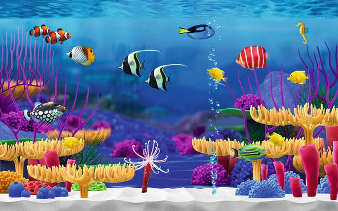
For this lesson, go to the book URL, click chapter7, click images, click fish.jpg, click the Download button, right-click inside the image, and click Save image as… to save it on your computer. Drag and drop the image to your Google Drive Colab Notebooks folder. Repeat the same process for the happy_moon.jpg image.

Mount Google Drive
Click the URL, choose a Google account, click Allow, copy the authorization code and paste it into Colab in the textbox Enter your authorization code:, and press the Enter key on your keyboard.
Copy Images to Google Drive
Before executing the code in this section, be sure that you have the fish.jpg and happy_moon.jpg images in the Colab Notebooks directory on your Google Drive!
Check your Google Drive account to verify the proper path. We saved the images to the Colab Notebooks directory, which is recommended. If you save them somewhere else, you must change the paths accordingly.
Load, scale, and display images
All is well so far.
Check Image Shapes
For machine learning applications, images must be of the same shape.
Uh-oh! Shapes are not the same! What do we do?
Resize Images
Now, all four images have size of (427, 640, 3).
Success! We resized the new images to correspond to the original ones.
Create a Batch of Images
Now, we have a batch of four 427 × 640 color images. RGB color is indicated by the 3 dimension.
Create Filters
Let’s create two simple 7 × 7 filters. We want our first filter to have a vertical white line in the middle and our second to have a horizontal white line in the middle. Filters are used to extract features from images during the process of convolution. Typically, filters are referred to as convolutional kernels.
The zeros method returns a given shape and type filled with zeros. Since variable ck is filled with zeros, all of its pixels are black. Remember that pixel image values are integers that range from 0 (black) to 255 (white).
So ck is a 4D tensor that contains two 7 × 7 convolutional kernels with three channels. The filters must have three channels to match the color images in the batch of images we created.
The code changes the intensity of select pixels to get a vertical white line and a horizontal white line.
Plot Convolutional Kernels
Convolutional kernel plots
We see that the vertical and horizontal white lines (or convolutional kernels) are in position. So we have successfully created two simple convolutional kernels.
Apply a 2D Convolutional Layer
The tf.nn.conv2d method computes a 2D convolution given 4D input and convolutional kernel tensors. We set strides equal to 1. A stride is the number of pixels we shift the convolutional kernels over the input matrix during training. With strides of 1, we move the convolutional kernels one pixel at a time. We set padding to SAME. Padding is the number of pixels added to an image when it is being processed by the CNN. For example, if padding is set to zero, every pixel value that is added will be of value zero. Padding set to SAME means that we use zero padding.
After applying the convolutional layer, the variable outputs contains the feature maps based on our images. Since each convolutional kernel creates a feature map (and we have two convolutional kernels), each image has two feature maps.
Visualize Feature Maps
Feature maps plot
Since we have two convolutional kernels and four images, the convolutional layer produces eight feature maps. Just multiply 2 by 4! So we have two feature maps for each image. Wow! With two simple convolutional kernels, we were able to extract excellent facsimiles of our batch of images by applying a single convolutional layer.
CNN with Trainable Filters
We just manually defined two convolutional kernels. But, in a real CNN, we typically define convolutional kernels as trainable variables so the neural net can learn the convolutional kernels that work best.
We create a Conv2D layer with 32 convolutional kernels. Each convolutional kernel is a 3 × 3 tensor indicated by kernel_size. We use strides of 1 both horizontally and vertically. Padding is SAME. Finally, we apply relu activation to the output.
Convolutional layers have quite a few hyperparameters including number of filters (or convolutional kernels), height and width of convolutional kernels, strides, padding type, and activation type. To get the best performance, we can tune the hyperparameters. But tuning is an advanced topic that we believe is not appropriate for an introductory book. Instead, we provide fundamental examples that you can practice to develop practical skills.
Building a CNN
Although a CNN is a sequential neural net, it does differ from a feedforward sequential neural net in two important ways. First, it has a convolutional base that is not fully connected. Second, it has a pooling layer to reduce the sample size of feature maps created by each convolutional layer. We still use a fully connected layer for classification.
We begin this experiment by loading a dataset of color images. We continue by preparing the data for TensorFlow consumption. We then build and test a CNN model. The dataset we use is cifar10. We previously modeled this dataset with a feedforward model, but our results were horrible. So we want to show you how much better a CNN works with complex color images.
Load Data
Since we already have info from the train set, we don’t need it again for the test set.
Train and test shapes are 32 × 32 × 3. So each image is a 32 × 32 three-channel image. The 3 dimension informs the model that images are RGB color.
Display Information About the Dataset
We see the name, description, homepage, and shapes and datatypes of feature images and labels. We also see that the dataset has 60,000 images with train and test splits of 50,000 and 10,000, respectively.
Extract Class Labels
Display Samples
Build a Custom Function to Display Samples
Function to display samples
The function retrieves images and label names. It then displays the image with its label name and index. The index is the class label as a number.
Change the color by adjusting indx between 0 and 5. Change the number of samples displayed by adjusting samples. Peruse the following URL to learn more about colormaps: https://matplotlib.org/3.1.0/tutorials/colors/colormaps.html.
Build a Custom Function to Display a Grid of Examples
Processed examples from the train set
To enable image plotting, we remove (or squeeze) the 3 dimension from the image matrix.
Function to display a grid of examples
Voilà!
Pinpoint Metadata
Build the Input Pipeline
Build the input pipeline
We build the input pipeline by shuffling train data, batching, scaling, caching, and prefetching. We scale images by mapping with a lambda function. Adding the cache method increases performance on a TFDS because data is read and written only once rather than during each epoch. Adding the prefetch method is a good idea because it adds efficiency to the batching process. That is, while our training algorithm is working on one batch, TensorFlow is working on the dataset in parallel to get the next batch ready. So prefetch can dramatically improve training performance.
Create the Model
Begin with a relatively robust CNN model because it is the only way to get decent performance from complex color images. Don’t be daunted by the number of layers! Remember that a CNN has a convolutional base and fully connected network. So we can think of a CNN in two parts. First, we build the convolutional base that includes one or more convolutional layers and pooling layers. Pooling layers are included to subsample the feature maps outputted from convolutional layers to reduce computational expense. Next, we build a fully connected layer for classification.
- 1.
Import libraries.
- 2.
Clear previous models.
- 3.
Create the model.
Build the model
The first layer is the convolutional base, which uses 32 convolutional kernels and kernel size of 3 × 3. We use relu activation, same padding, and strides of 1. We also set shape at 32 × 32 × 3 to match the 32 × 32-pixel images. Since images are in color, we include the 3 value at the end. Next, we include a max pooling layer of size 2 (so it divides each spatial dimension by a factor of 2) to subsample the feature maps from the first convolutional layer. We then repeat the same structure twice, but increase the number of convolutional kernels to 64. It is common practice to double the number of convolutional kernels after each pooling layer.
We continue with the fully connected network, which flattens its inputs because a dense network expects a 1D array of features for each instance. We need to add the fully connected layer to enable classification of our ten labels. We continue with a dense layer of 64 neurons. We add dropout to reduce overfitting. The final dense layer accepts ten inputs to match the number of labels. It uses softmax activation.
Model Summary
Parameters are the number of learnable weights during training. The convolutional layer is where the CNN begins to learn. But calculating parameters for a CNN is more complex than a feedforward network.
The first layer is a convolutional layer with 32 neurons acting on the data. Filter size is 3 × 3. So we have a 3 × 3 × 32 filter since our input has 32 dimensions (or neurons) for a total of 288. Multiply 288 by 3 to account for the 3D RGB color images for a total of 864. Add 32 neurons at this layer to get a total of 896 parameters.
There are no parameters to learn at the pooling layers. So we have 0 parameters.
The second convolutional layer has 64 neurons acting on the data. Filter size is 3 × 3. So we have a 3 × 3 × 64 filter since we have 64 dimensions for a total of 576. Multiply 32 neurons from the previous convolutional layer by 576 to get a total of 18,432. Add 64 neurons at this layer to get a total of 18,496 parameters.
The third convolutional layer has 64 neurons acting on the data. Filter size is 3 × 3. So we have a 3 × 3 × 64 filter since we have 64 dimensions for a total of 576. Multiply 64 neurons from the previous convolutional layer by 576 to get a total of 36,864. Add 64 neurons at this layer to get a total of 36,928 parameters.
The fully connected dense layer is calculated as before. We get 262,144 by multiplying 4,096 neurons at this layer by 64 neurons from the previous layer. Add 64 neurons at this layer to get a total of 262,208 parameters.
The output layer has 650 parameters by multiplying 64 neurons from the previous layer by 10 at this layer and adding 10 neurons at this layer. Whew!
Model Layers
Compile the Model
Train the Model
Although our model is not state of the art, we do much better than we did with a feedforward net.
Generalize on Test Data
Visualize Training Performance
Visualization of training performance
Predict Labels for Test Images
Wrap the predict method with the argmax method to get predicted labels directly rather than generating probability arrays.
First five actual labels
Get the first batch of images. Since we set batch size at 128, we get the first 128 images. Slice the first five images from the batch. Convert to label names.
Compare pred_labels to actual_labels to get an idea of prediction performance.
Build a Prediction Plot
Take samples from the test set
Build a Custom Function
Function to display results
Titles in red indicate misclassifications.
Build a CNN with Keras Data
Although loading data as a TFDS is recommended, Keras is very popular in industry. So let’s build a model from keras.datasets.
Create Variables to Hold Train and Test Samples
Create variables to hold train and test data
Display Sample Images
It’s always a good idea to display some images. In this case, we display 30 images from the training dataset. Visualization allows us to verify that images and labels correspond. That is, a frog image is labeled as a frog and so on.
Display sample images
Create the Input Pipeline
Build the input pipeline by scaling images and slicing them into TensorFlow consumable pieces. Continue by shuffling (where appropriate), batching, and prefetching.
Build the input pipeline
Create the Model
Create the model
Compile and Train
Compile and train the model
Predict
Visualize Results
Visualize training performance results
Epilogue
Many improvements to the fundamental CNN architecture have been developed over the past few years that vastly improve prediction performance. Although we don’t cover these advances in this lesson, we believe that we provided the basic foundation with CNNs to help you comfortably work with these recent advances and even the many advances to come in the future.