CHAPTER 5

Valuing High-Yield Bonds: A Business Modeling Approach

Thomas S. Y. Ho^a,*and Sang Bin Lee^b

1. INTRODUCTION

There has been much research on the valuation of corporate bonds with credit risks in the past few years. The impetus of the research may be driven by a number of factors. Recently, there has been a surge of bonds facing significant credit risks, as a result of the downturn of the economy after the burst of the new economy bubble. For example, in the telecommunication sector, a number of firms have declared default because of the excess supply of telecommunication infrastructure and financial obligations. Another reason is the impending change in regulations in risk management. Increasingly, regulators are demanding more disclosure of risks from the financial institutions and the measures of credit risks in the firm's investment portfolio. The financial disclosure would lead to the examination of the adequacy of capital for the firms. Finally, the credit risk model is important for the use of a number of recent financial innovations. These innovations include collateralized debt obligations, credit default swaps, and other credit derivatives that have demonstrated significant growths in the past few years. The credit risk model is important in determining these securities' values and managing their risks.

Valuing bonds with credit risk must necessarily be a complex task. A high-yield bond tends to have the business risk of the bond's issuer. And, therefore, the valuing of a high-yield bond may be as involved as valuing the equity of the issuer. Indeed, both the bonds and the equity of a firm are contingent claims on the firm value.

One approach to valuing a high-yield bond is that of Merton (1974). The model views the firm's equity as a call option on the firm value and applies the Black-Scholes model to value a corporate bond. This approach does not require the investors to know the profitability of the firm and the market expected rate of return of the firm. The model needs to know only the prevailing firm value and its stochastic process. In essence, according to the Merton model, a defaultable bond is a default-free debt embedded with a short position of a put option on the firm value, with the strike price equaling the face value of the debt and the time to expiration equaling the maturity of the bond. More generally, models that view a high-yield bond as a bond with an embedded put option are called structural models.

There are many extensions of the Merton model. One general extension is the use of a trigger default barrier that specifies the condition for default. For example, the Longstaff and Schwartz¹ (1995) model allows the firm to default at any time whenever the firm value falls below a barrier. This approach views that a bond has a barrier option embedded in a default-free bond. This model has been extended by Saa-Requejo and Santa-Clara (1999), allowing for the stochastic strike price; Briys and de Varenne (1997) allow the barrier to be related to the market value of debt. Such extensions assume the stochastic firm value captures all of the business risk of the firm. They do not model the business of the firm and they, in particular, ignore the importance of the negative cash flows of a firm in triggering the event of default.

To avoid such shortcomings, the Kim et al. (1993) model assumes that the bondholders get a portion of the face value of the bond at default, which is based on the lack of cash flow to meet obligations. They define the default trigger point as a net cash flow at the boundary, when the firms cannot pay for the interests and dividends. Brennan and Schwartz use the real option approach to determine the firm value as a contingent claim on the business risk. Using this approach, they model the value of a mining company. The real option valuation approach extends the Merton model to specify the business model of a firm and, therefore, the approach values the corporate bonds as compound options on the business risks.

This chapter takes this real option approach to value the high-yield bonds. Specifically, we model the business of the firm and its operating cash flows contingent on the business risks. Using the structural model's compound option concept, we determine the default conditions of a firm, given its capital structure and the business model. In essence, our approach endogenizes the trigger default barrier of the firm using the firm's business model and the capital structure.

Specifically, we propose that a firm's fixed operating costs play a significant role in triggering default of the bond's debt. When the firm has a negative operating income that cannot be financed internally, the firm must necessarily seek funding in the capital markets. However, if the firm value is low in relation to all of its future financial obligations, then the firm may not be able to fund the negative operating income, leading to default. Indeed, some bonds are considered risky because of the firm's high operating leverage, even though the financial leverage may be low.

In comparison with the structural models in the research literature, our model suggests that the firm value stochastic process is not a simple lognormal process. Instead, the firm value follows an “option” price process. And the debt is not a risk-free bond embedded with a put option. It is embedded with a compound option and it is a “junior debt” to the fixed costs.

This approach has broad implications to debt valuation. Our model suggests that the pricing of defaultable bonds must include more financial information of a firm: in particular, the financial and operating leverage of the firm. The model allows for the firm to default before the bond matures by allowing the negative cash flow to trigger a default. Since the model does not require an exogenously specified trigger default function, but solves for the default condition using the option pricing approach, we can use the model to price the bonds using the firm's financial statements, which are widely available. Therefore, the model can be tested empirically.

In this chapter, we provide some empirical evidence to support the validity of the model. While this chapter provides a simple model, we show that the approach is very general. Extensions of the model will be left for future research.

The chapter proceeds as follows. We describe the model in Section 2, presenting the assumptions made in the model. For the clarity of the exposition, in Section 3, we provide a numerical example, showing how the model can be used to market available data. Section 4 presents some empirical evidence on the validity of the model. Section 5 discusses some of the implications of the model and, finally, Section 6 provides the conclusions.

2. SPECIFICATION OF THE MODEL

This section presents the assumptions of the model. Similar to the Merton model, we assume that the market is perfect, with no transaction costs. We assume that there are corporate and personal taxes such that the assumptions are consistent with the Miller model. The corporate tax rate of the firm is assumed to be τ_c. In this world, the capital structure does not affect the value of the firm. We use a binomial lattice framework to construct the risk processes.

We assume that the yield curve is flat and is constant over time at an annual compounding rate of r_f. The bond valuation model is based on a real option model. Specifically, we begin with the description of the business risk of the firm by depicting the primitive firm lattice V^p(n, i). We then build the firm value lattice V(n, i), which includes some considerations of a valuation of a firm: fixed costs and taxes. Finally, we use the firm value lattice to analyze all of the claims on the firm value, based on the Miller and Modigliani (MM) framework.

2.1 Primitive Firm

The firm, the equity, the debt, and all other claims on the firms are treated as the contingent claims to the primitive firm. The primitive firm is the underlying “security” to all these claims and it captures the business risk of the firm.

We begin with the modeling of the business risk. We assume that the firm has a fixed capital asset and the capital asset generates uncertain revenues. The gross return on investment (GRI) is defined as the revenue generated per $1 of the capital asset. GRI is a capital asset turnover ratio. In this simplified model, we consider a firm is endowed with a capital asset that does not depreciate and can generate perpetual revenues.

Specifically, we assume that GRI follows a binomial lattice process that is lognormal (or multiplicative) with no drift, a martingale process, where the expected GRI value at any node point equals the realized GRI at that node point (n, i), where n is the number of time steps and i denotes the state of the world. Specifically,

with probability q, where 0 < q < 1 and

with probability 1 – q.

The market probability q is chosen so that the expected value of the risk over one period is the observed risk at the beginning of each step. That is, the risk follows a martingale process stated below:

where

σ being the volatility of the risk driver.

We assume that the MM theory can be extended to the multi-period dynamic model described above. In this extension, we assume that all of the individuals make their investment decisions and trading at each node on the lattice. These activities include the arbitrage trades described in the MM theory. The results of the theory apply to each node. Therefore, there is a cost of capital ρ at each node dependent on the business risk and not on the risk of the firm's free cash flows, which depend on the operating leverage.

The cost of capital ρ of a sector is the required rate of return for that sector business risk, assuming that the firm has no fixed costs. By way of contrast, the cost of capital of MM theory assumes a particular firm, taking the operating leverage as given. The cost of capital of a firm according to the MM theory reflects the risk of the free cash flows of the firm. Here, we extend this concept of MM theory to a business sector and use a firm with no operating leverage as the benchmark for comparison.

Since the production process is the same at each node on the lattice, the firm risk is the same at each node. For this reason, we will assume that the cost of capital is constant in all states and time. According to the MM theory, the firm value is the present value of all of the firm's free cash flow along all of the paths on the lattice. In particular, the lattice of the primitive firm value is given as

where m is the gross profit margin.

By the definition of the binomial process of the gross return on investment, we have

Further, since the cost of capital of the firm is ρ, the firm pays a cash dividend of

Therefore, the total value of the firm V_u^p, an instant before the dividend payment in the up state, is

Similarly, the total value of the firm V_d^p, an instant before the dividend payment in the down state, is

Then, the risk neutral probability P is defined as the probability that ensures the expected total return is the risk-free return:

Substituting V^p, V_u^p, V_d^p into the equation above and solving for P we have

where

Note that as long as the volatility and the cost of capital are independent of the time n and state i, the risk-neutral probability is also independent of the state and time, and is the same at each node point on the binomial lattice. We have now changed the measure from market probability to the risk-neutral probability. We will use this risk-neutral probability to determine the values of the contingent claims.

2.2 The Firm Value

We assume that the firm pays out all of the free cash flows. Let the fixed cost be FC, which is constant over time and state. In the case of negative cash flow, we assume that the firm gets tax credits, and the firm raises the funds from equity. This assumption is quite reasonable since tax credits can carry forward for over 20 years; the government in essence participates in the business risks of the firm and it should not affect the basic insight of the model. The cash flow is the revenue net of the operating costs, fixed costs, and taxes:

This model assumes that the firm has no growth over this time horizon. This assumption is quite reasonable because the high-yield companies often cannot implement growth strategies. Further, the model can be extended in a straightforward manner to incorporate growth for a firm when growth is important to its bond pricing. Ho and Lee (2004) provide an extension of the model with growth, allowing for optimal investment decisions.

The terminal value at each state in the binomial lattice at the horizon date has four components: the present value of the gross profit; the present value of the fixed costs, which takes the possibility of future default into account; the present value of the tax that is approximated as a portion of the pretax firm value; and, finally, the cash flows of the firm at each node point.

Following the Merton (1974) model, we assume that the firm pays no dividends after the planning period and the primitive firm follows a price dynamic described below:

where dZ is the Wiener process.

The present value of the fixed costs is determined as a hypergeometric function, according to Merton (1974), since we assume that the firm can go default in the future and the fixed costs are not paid in full.

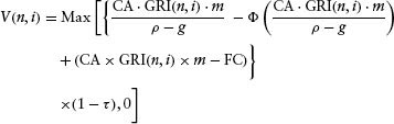
The lattice of the firm value is determined by rolling back the firm values, taking the cash flows into account. The firm value at the terminal period at each node is

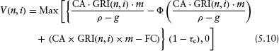
where Φ(g) is the present value of the perpetual risky fixed cost, and Φ(g) is the valuation formula of the perpetual debt given by Merton(1973) presented in the Appendix.

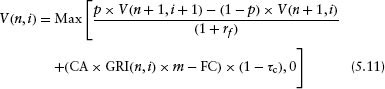
In the intermediate periods, the firm value is determined by backward substitution:

2.3 Debt Valuation and Market Capitalization

We assume that the firm value is independent of the debt level. The value of the bond is determined by the backward substitution approach. The stock lattice is the firm lattice net of the bond lattice. We first consider the terminal conditions for the bond to be Min(debt obligation at T, firm value at T).

We then conduct the backward substitutions such that we apply the valuation rule at each node point: Min(backward substitution bond value + bond cash flow, firm value).

Following the standard methodology, the rolling back procedure leads to the value of the debt at the initial value. The market capitalization of the firm is the firm value net of the debt value.

3. A NUMERICAL ILLUSTRATION

We assume that the yield curve is flat and is constant over time at a 4.5% annual compounding rate. The market premium is defined as the market expected return net of the risk-free rate, which is assumed to be 5%. The tax rate of the firm is 30%, which is assumed to be the marginal tax rate. The model is based on a five-step binomial lattice. It is a one-factor model, with only the business risk. The model is arbitrage free relative to the underlying values of a firm that bears all the business risks of the revenues.

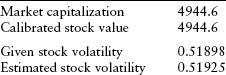
We use one firm, Hilton Hotels, in the sector of consumer and lodging, as an example to illustrate the implementation of the model. On the evaluation date October 31, 2002, the market capitalization is reported to be $4,944 million, the stock volatility estimated to be the 1-year historical volatility of Hilton's stock, is 51.9%, and the stock beta is 1.255. Using the capital asset pricing model, we estimate that the expected rate of return of the stock

The financial data are given from the financial statements as follows. The revenue is $2834 million, with the operating cost of $1,542 million and fixed cost of $726 million. The capital asset is $7,714 million with the long-term debt of $5,823 million and interest costs of $357 million. Using these data, we can calculate

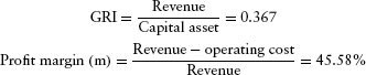
3.1 The GRI Lattice

To generate the GRI lattice, we have to assume the sector cost of capital and the volatility initially to begin the iterative process. Let us assume the cost of capital spread to be 1.57% and the sector volatility 11.54%. The assumed data are an initial input for the nonlinear optimization procedure. Using the assumed data, we can calculate the expected returns of the sector (ρ):

We can now determine the primitive firm lattice based on the model:

We can also calculate the cash flow of the primitive firm at each node point. The lattice of cash flow at each state, based on the capital asset of $7,714 million, is

The risk neutral probability is

3.2 The Firm Value

The fixed costs of the firm stay the same. The gross margin also remains constant. The firm defaults when the firm cannot finance the fixed costs. All excess cash flows are paid out.

A lattice of cash flow at each state is developed. At each node, the cash flow is the revenue net of the operating costs, fixed costs, and taxes;

The terminal value at each state is given below. By assuming that the long-term growth rate g is 1.57%, the firm value at the terminal period at each node is

where Φ(g) is given in the Appendix. At the terminal date, the time horizon where n = 5, the firm value for each node is

Now, we roll back the firm value from the terminal value, taking the cash flows into account. In the intermediate periods, the firm value is determined by backward substitution:

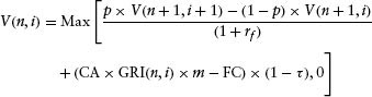
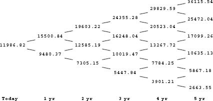
FIGURE 5.1 Lattice of the firm value.

The resulting lattice is shown in Figure 5.1.

3.3 Debt Valuation and Market Capitalization

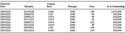
The debt structure of Hilton Hotels is somewhat complicated, with eight bonds, and is shown in Table 5.1.

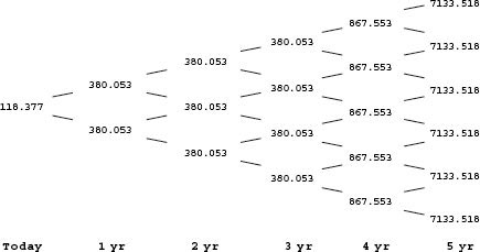
Using the debt structure given above, we can calculate the promised cash flow of the bonds, which are $118.377 thousand at year 0, $380.053 thousand for the period from year 1 to year 3, and $867.553 and $7,133.518 thousand at years 4 and 5, respectively.

We use the lattice of the firm model, the lattice of the debt cash flow, and the standard backward substitution procedure to determine the debt value. The resulting lattice of the debt is shown in Figure 5.2.

Table 5.1 Debt Package of Hilton Hotels

FIGURE 5.2 Debt cash flows.

The market capitalization value is the firm value net of the debt value. Finally, given that the bond price is $5,818 million, the internal rate of return is 9.26%, and the credit risk spread, which is the internal rate of return net of the risk-free rate, is 476 basis points. From the two nodes of the first period of the stock lattice and the sector lattice, the lattice of the primitive firm, we can calculate the stock volatility and the sector volatility.

3.4 Calibration

Recall that this procedure thus far has assumed the following input data: long-term growth rate of the firm g, sector volatility σ_p, and sector expected excess return ρ under market probability. There are in essence three unknowns. These data are not observed directly. They are just initial data to enable us to proceed with the algorithm in determining the bond value.

However, the model derives the following values: market capitalization and the stock volatility, which we can directly observe. Further, note that the excess return of the stock can be determined by the capital asset pricing model and by the equation below, which is based on the market price of risk of a contingent claim. This provides the third constraint to the nonlinear search with three control variables.

Therefore, we can use a nonlinear estimation procedure in perturbing the assumed data, the long term growth rate and the sector volatility, such that the model-derived value equals the observed values.

Market capitalization and stock volatility = observed market capitalization and stock volatility.

4. EMPIRICAL EVIDENCE

We use an example of McLeodUSA to demonstrate empirically the relationship between the market capitalization and the bond package value. We show that as the market capitalization of the firm falls, the bond package value would also fall. However, the bond value falls more precipitously than the market capitalization as the firm approaches bankruptcy.

We also show that the Merton model of the corporate bond can explain much of this relationship between the market capitalization and the bond value. But the model tends to understate the acceleration of the fall in the bond prices when the market capitalization falls below a certain value.

We use our model to explain this relationship between the market capitalization and the bond package value. Specifically, we assume that the gross return on investment declines, leading the fall in the market capitalization and the bond value. It is quite reasonable to make this assumption. A source of the financial problem of McLeodUSA was that the expectation of the demand for communication had been falling along with an excess supply of communication networks. As a result, the market revised its expectations of the returns of the McLeodUSA assets, and hence the fall of GRI.

We use the calibrated business model of McLeodUSA. The sector volatility and the implied long-term growth rate are estimated to be 0.0935 and 0.0332, respectively. Further, we add a spread to the Treasury curve in dis-counting the bond such that the bond price equals the observed price initially. The use of a spread is reasonable because we have discussed that bonds tend to have a liquidity spread and a risk premium (a market price of risk for the model risks not captured by the model) in predicting defaults. Referring to Figure 5.1, the results show that the proposed model provides relatively better explanatory power of the observations than the Merton model. In particular, using the proposed model, we predict the precipitous fall of the bond value better than when we use the Merton model.

The empirical evidence can be explained intuitively. McLeodUSA is a communication company that has significant operating costs. Note that the debts outstanding do not mature in the next 3 years and there is no immediate maturity of crisis for the firm in the short run. However, because of the significant fixed cost resulting in losses of the operation, the firm's operation has to be supported by external financing. When the market revises downward on the returns of the assets, the market capitalization falls, leading to the situation where McLeodUSA fails to have access to the capital market to fund its negative operating costs. In essence, the firm defaults on its operating costs, something that the Merton model would not have considered (Figure 5.3).

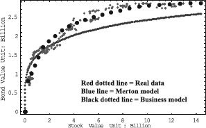
FIGURE 5.3 Stock value versus bond value of McLeodUSA.

5. IMPLICATIONS OF THE MODEL

The proposed model is an extension of Merton's structural model, where we have used the relative valuation approach to solve for valuation of the market value of debt. Therefore, we have not used any historical estimation of the survival rate of the bonds, which require the model to hypothesize the appropriate market discount rate for the expected cash flow. Also, this approach does not require any assumption of the recovery ratio, which is endogenous in the structural model.

When compared with the Merton model, this model predicts that the firm can default without the crisis of maturity. The default event can be triggered by the fixed costs. This model can explain the market observation that some firm has a low credit rating and trades with a high-yield spread, even though the market debt-to-equity ratio is low.

This model of the bond price is sensitive to the stock price, as with the Merton model. The main advantage of the proposed model is that it allows us to use more detailed information about the firm, and therefore the bond valuation model is more realistic. Finally, the model is empirically testable. The financial data, bond yield spreads, and stock prices are relatively accessible.

6. CONCLUSIONS

This chapter proposes a valuation of bonds with credit risks. The main contribution of the chapter is to introduce the concept of a primitive firm. The primitive firm has neither operating leverage nor financial leverage. Given the risk class of this primitive firm, we can determine the value of a firm with operating and financial leverage as a contingent claim to the primitive firm.

This approach enables us to introduce the business model of a firm in the high-yield bond valuation. Relating the high-yield bond pricing to the firm's business is standard in practice, and this approach provides a more robust analytical framework for practitioners in the high-yield area.

The model provides intuitive insights into the high-yield bond behavior. For example, the model shows that the fixed costs of the firm can be viewed as the “perpetual debt” of the firm, senior to the financial debt obligations. Such a treatment of the fixed costs significantly affects the probability distribution in the event of default of a firm and the valuation of the debt. Furthermore, it shows that the bond price is more sensitive to the market capitalization. As the market capitalization falls, the firm with significant fixed costs would fall precipitously with the market capitalization, before the event of default becomes imminent. For this reason, the model shows that the relationship of the probability of default and the bond price must also depend on the fixed cost level. This may explain the observation that the rating of the bond tends to lag behind the market pricing of the bonds. Since the bond rating measures the probability of default, which is different from the bond pricing as this model shows, the extent of the lag must depend on the firm's operating leverage.

This also suggests that models that use bond value or market capitalization to predict the probability of default can also be erroneous. We show that the bond value depends on both the recovery ratio and the probability of default. Since the recovery ratio depends on the firm's operating leverage, the firm default probability cannot be related simply to the market capitalization or the bond price without taking the firm's business model into account.

Finally, the proposed model shows that the use of a primitive firm can have broad implications for future research. The study of the primitive firms for different market sectors will enable us to better understand the high-yield bond valuation.

ACKNOWLEDGMENTS

We would like to thank Yoonseok Choi, Hanki Seong, Yuan Su, and Blessing Mudavanhu for their assistance in developing the models and in our research. We also would like to thank Owen Graduate School of Management at Vanderbilt University, seminar participants of Management for valuable comments. Any errors are ours.

APPENDIX

The valuation formula of the perpetual debt was given by Merton(1973):

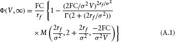
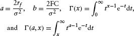
where V is the primitive firm value, FC the fixed cost per year, r_f the risk-free rate, Γ the gamma function (defined below), σ the standard deviation of GRI, and M(·) the confluent hypergeometric function (defined below).

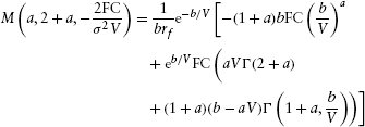
where

NOTES

1. See p. 792, Assumption 4, Longstaff and Schwartz (1995).

REFERENCES

Briys, E. and de Varenne, F. (1997). “Valuing Risky Fixed Rate Debt: An Extension.” Journal of Financial and Quantitative Analysis 32(2), 239–248.

Ericsson, J. and Reneby, J. (1998). “A Framework for Valuing Corporate Securities.” Applied Mathematical Finance 5(3), 143–163.

Ho, T. S. Y. and Lee, S. B. (2004). The Oxford Guide to Financial Modeling. NewYork: Oxford University Press.

Longstaff, F. A. and Schwartz, E. M. (1995). “A Simple Approach to Valuing Risky Fixed and Floating Rate Debt.” Journal of Finance 50(3), 789–819.

Saá–Requejo, J. and Santa-Clara, P. (1999). “Bond Pricing with Default Risk”. Working Paper, University of California, Los Angeles.

Shimko, D., Tejima, N. and van Deventer, D. (1993). “The Pricing of Risky Debt when lnterest Rates are Stochastic.” Journal of Fixed Income 3(2).

Vasicek, O. (1977). “An Equilibrium Characterization of the Term Structure.”Journal of Financial Economics 5, 177–188.

Keywords: High yield bonds; business model; structural model; contingent claim theory; operating leverage; default

---

^a Thomas Ho Company, Ltd., New York, NY, USA.

^b School of Business Administration, Hanyang University, Seoul, 133–791, Korea.

^*Corresponding author. Thomas Ho Company, Ltd., 55 Liberty Street, 4B, New York, NY, 10005–1003, USA. Tel.: 1–212–571–0121; e-mail: [email protected].