9. Analysis of the Energy Consumed by Appliances

Overview

This chapter aims to display the application of general data analysis techniques to a specific use case—analyzing the energy consumed by household appliances. By the end of this chapter, you will be able to analyze individual features of the dataset to assess whether the data is skewed. You will also be equipped to perform feature engineering by creating new features from existing ones, and also to conduct Exploratory Data Analysis (EDA) and design informative visualizations.

Introduction

In the previous chapter, we took a look at the retail industry through the dataset of an online retail store based out of the UK. We applied a variety of techniques, such as breaking down the date-time column into individual columns containing the year, month, day of the week, hour, and so on, and creating line graphs to conduct a time series analysis to answer questions such as 'Which month was the most popular for the store?'

This chapter guides you through the data-specific analysis of a real-world domain and situation. This chapter focuses on a dataset containing information regarding the energy consumption of household appliances. The true goal of this dataset is to understand the relationships between the temperature and humidity of various rooms of a house (as well as outside the house) to then predict the energy consumption (usage) of appliances. However, in this chapter, we are just going to analyze the dataset to reveal patterns between the features.

This dataset has been retrieved from the UCI Machine Learning Repository. The data consists of temperature and humidity values for several rooms in a house in Belgium, monitored by wireless sensors. The data regarding the energy used by the lights and appliances was recorded by energy meters. The temperature, humidity, and pressure values for outside the house were procured from the nearest airport weather station (Cheivres Airport, Belgium). The two datasets have been merged together based on date and time.

Note

The original data can be found here: https://archive.ics.uci.edu/ml/datasets/Appliances+energy+prediction#.

You can also find the dataset in our GitHub at: https://packt.live/3fxvys6.

For further information on this topic, refer to the following: Luis M. Candanedo, Veronique Feldheim, Dominique Deramaix, Data-driven prediction models of energy use of appliances in a low-energy house, Energy and Buildings, Volume 140, 1 April 2017, 81-97, ISSN 0378-7788

To understand the dataset further, let's take a closer look.

Note

All the exercises and activities are to be done in the same Jupyter notebook, one followed by the other.

Exercise 9.01: Taking a Closer Look at the Dataset

In this exercise, you will load the data and use different viewing methods to better understand the instances and features. You will also check for missing values, outliers, and anomalies and deal with them through imputation or deletion if required:

1. Open a new Jupyter notebook.
2. Import the required packages:

   import pandas as pd

   import numpy as np

   import seaborn as sns

   import matplotlib.pyplot as plt

   import plotly.express as px

3. Read the data from the link using pandas' read_csv function and store it in a DataFrame called data:

   data = pd.read_csv('https://raw.githubusercontent.com/'

                      'PacktWorkshops/The-Data-Analysis-Workshop/'

                      'master/Chapter09/Datasets/'

                      'energydata_complete.csv')

4. Print the first five rows of data using the .head() function:

   data.head()

   A truncated version of the output is shown below:

   

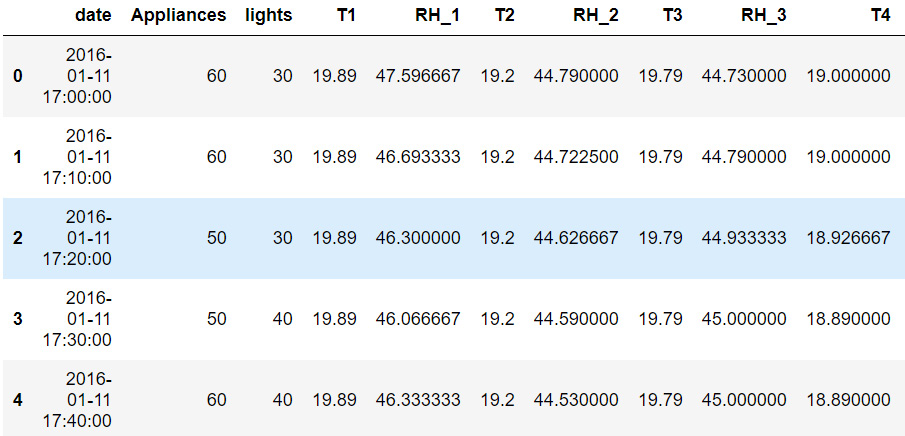
   Figure 9.1: The first five rows of data

5. Check to see if there are any missing values. Use the .isnull() function to check for missing values in each column, and the .sum() function to print the total number of missing values per column:

   data.isnull().sum()

   The output will be as follows:

   

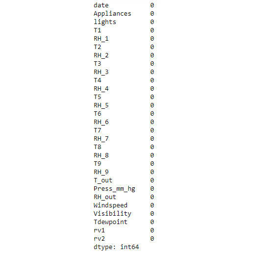
   Figure 9.2: The number of missing values per column

   The preceding output indicates that there are no missing values. This makes your job easier as now you don't need to figure out how to deal with them.

6. Change these column names in the current DataFrame to make them less confusing. If you click on the dataset link provided in the first Note box in this chapter, you'll see a section titled Attribute Information. This section elaborates on each column name to tell us what the values of that column actually mean. Use this information to rename the columns so that they're easier to understand. Rename these columns in a new DataFrame called df1:

   df1 = data.rename(columns = {'date' : 'date_time',

                                'Appliances' : 'a_energy',

                                'lights' : 'l_energy',

                                'T1' : 'kitchen_temp',

                                'RH_1' : 'kitchen_hum',

                                'T2' : 'liv_temp',

                                'RH_2' : 'liv_hum',

                                'T3' : 'laun_temp',

                                'RH_3' : 'laun_hum',

                                'T4' : 'off_temp',

                                'RH_4' : 'off_hum',

                                'T5' : 'bath_temp',

                                'RH_5' : 'bath_hum',

                                'T6' : 'out_b_temp',

                                'RH_6' : 'out_b_hum',

                                'T7' : 'iron_temp',

                                'RH_7' : 'iron_hum',

                                'T8' : 'teen_temp',

                                'RH_8' : 'teen_hum',

                                'T9' : 'par_temp',

                                'RH_9' : 'par_hum',

                                'T_out' : 'out_temp',

                                'Press_mm_hg' : 'out_press',

                                'RH_out' : 'out_hum',

                                'Windspeed' : 'wind',

                                'Visibility' : 'visibility',

                                'Tdewpoint' : 'dew_point',

                                'rv1' : 'rv1',

                                'rv2' : 'rv2'})

7. Print the first five rows of df1 using the .head() function:

   df1.head()

   A truncated version of the output is shown below:

   

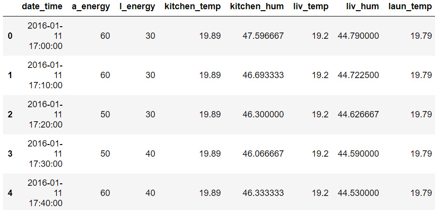
   Figure 9.3: The first five rows of df1

   This table looks easier to understand. The a_energy and l_energy columns are the energy consumed by the appliances and lights respectively and are both in Wh (watt-hour). The temperature columns are all in degree Celsius and humidity columns are in %. The pressure column is in mm Hg, the wind speed column is in meters per second, visibility is in kilometers, and Tdewpoint is in degree Celsius.

   A closer look at the date_time column tells us that there's a time interval of 10 minutes between each instance.

8. Print the last five rows of df1:

   df1.tail()

   The output will be as follows:

   

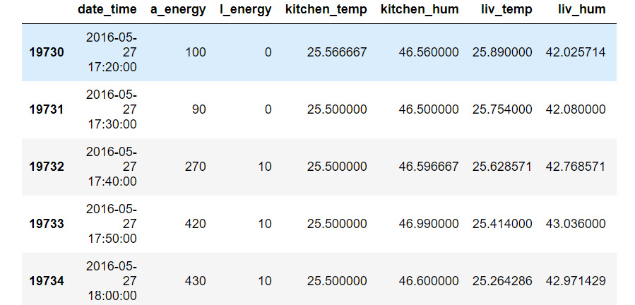
   Figure 9.4: The last five rows of df1

   Comparing the date_time columns in Figure 9.3 and Figure 9.4 shows us that this data has been collected over approximately 4.5 months—from January 11, 2016 to May 27, 2016.

   Now that we have an idea of what our data is about, let's check the values out.

9. Use the .describe() function to get a statistical overview of the DataFrame:

   df1.describe()

   The output will be as follows:

   

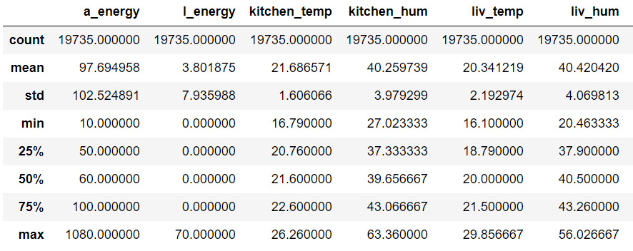
Figure 9.5: Overview of df1

Note

The output has been truncated for presentation purposes. The full output can be found here:

https://packt.live/34imyTx.

Note

To access the source code for this specific section, please refer to https://packt.live/34imyTx.

You can also run this example online at https://packt.live/3hAZqG0. You must execute the entire Notebook in order to get the desired result.

We can make a lot of observations based on the information present in Figure 9.5. These observations can help us determine whether our data requires deeper cleaning, preparation, and analysis, or whether it is fine and good to go.

For example, all the humidity and temperature columns seem fine; the minimum and maximum values seem reasonable and not extreme.

However, the two energy columns seem a bit odd. The a_energy column has a maximum value of 1,080, but the mean is around 97. This means that there are a few extreme values that might be outliers. The l_energy column has a 0 value for minimum, 25%, 50%, and 75%, and then has 70 as its maximum value. Something doesn't seem right here, so let's take a closer look.

Exercise 9.02: Analyzing the Light Energy Consumption Column

In this exercise, you will focus on the data present in one column of our DataFrame—l_energy, which explains the energy consumption of lights around the house:

1. Using seaborn, plot a boxplot for l_energy:

   lights_box = sns.boxplot(df1.l_energy)

   The output will be as follows:

   

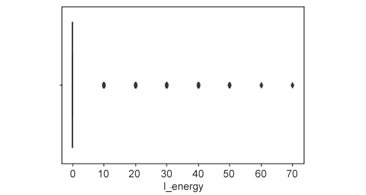
   Figure 9.6: Boxplot of l_energy

   This plot seems quite peculiar. It makes you wonder how many instances exist for each of these unique values.

2. Since you know that there are 8 unique Wh values present in the l_energy column, store these in a list:

   l = [0, 10, 20, 30, 40, 50, 60, 70]

3. Create an empty list called counts, which is where we'll store the number of instances per Wh:

   counts = []

4. Write a for loop that iterates over each value in l, calculates the total number of instances for each value in l, and appends that number to counts:

   for i in l:

       a = (df1.l_energy == i).sum()

       counts.append(a)

5. Print counts:

   counts

   The output will be as follows:

   [15252, 2212, 1624, 559, 77, 9, 1, 1]

   The preceding results show that the majority of the values present in l_energy are 0.

6. Plot a bar graph to better understand the distribution of the l_energy column using seaborn. Set the x axis as l (the Wh values) and the y axis as counts (the number of instances). Set the x-axis label as Energy Consumed by Lights, the y-axis label as Number of Lights, and the title as Distribution of Energy Consumed by Lights:

   lights = sns.barplot(x = l, y = counts)

   lights.set_xlabel('Energy Consumed by Lights')

   lights.set_ylabel('Number of Lights')

   lights.set_title('Distribution of Energy Consumed by Lights')

   The output will be as follows:

   

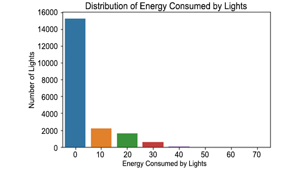
   Figure 9.7: Distribution of energy consumed by lights

   As you can see, most of the instances present in df1 have 0 Wh as the energy consumed by lights.

7. Calculate the percentage of 0 values in l_energy by dividing the number of instances with 0 Wh by the total number of instances in df1 and multiplying this by 100:

   ((df1.l_energy == 0).sum() / (df1.shape[0])) * 100

   The output will be as follows:

   77.28401317456296

   77% of the instances have 0 Wh. This renders the l_energy column quite useless because we can't possibly find any links between it and the other data. So, let's get rid of this column.

8. Create a copy of df1 called new_data:

   new_data = df1

9. Use the .drop() function to drop the l_energy column new_data. Set axis as 1 to tell the function that we want to drop a column, not a row, and set inplace as True:

   new_data.drop(['l_energy'], axis = 1, inplace = True)

10. Print the first five rows of new_data, using .head():

    new_data.head()

    The output will be as follows:

    

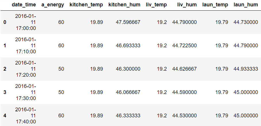
Figure 9.8: The first five rows of new_data

Now there's no l_energy column.

Note

To access the source code for this specific section, please refer to https://packt.live/3ee7U3K.

You can also run this example online at https://packt.live/3e9tSF5. You must execute the entire Notebook in order to get the desired result.

In this exercise, we successfully analyzed the l_energy column to understand the data pertaining to the consumption of energy of light fittings. We observed that a majority of the instances had a 0 Wh value for this column, which resulted in it being redundant. Therefore, we dropped the entire column from our DataFrame.

Activity 9.01: Analyzing the Appliances Energy Consumption Column

In this activity, you are going to analyze the a_energy column in a similar fashion to the l_energy column in Exercise 9.02, Analyzing the Light Energy Consumption Column. Please solve Exercise 9.01: Taking a Closer Look at the Dataset and Exercise 9.02, Analyzing the Light Energy Consumption Column before solving this activity.

1. Using seaborn, plot a boxplot for the a_energy column:

   The output will be as follows:

   

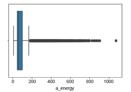
Figure 9.9: Box plot of a_energy

This box plot looks a little less weird than that of l_energy, but something is still off here. You can see that a majority of the values seem to lie between 50 Wh and 100 Wh. However, some values extend the upper bracket of 200 Wh and go beyond 1000 Wh. This seems odd. Check to see how many values extend above 200 Wh.

1. Use .sum() to determine the total number of instances wherein the value of the energy consumed by appliances is above 200 Wh.

   The output will be as follows:

   1916

2. Calculate the percentage of the number of instances wherein the value of the energy consumed by appliances is above 200 Wh.

   The output will be as follows:

   9.708639473017481

3. Use .sum() to check the total number of instances wherein the value of the energy consumed by appliances is above 950 Wh.

   The output will be as follows:

   2

4. Calculate the percentage of the number of instances wherein the value of the energy consumed by appliances is above 950 Wh.

   The output will be as follows:

   0.010134279199391943

   Only 0.01% of the instances have a_energy above 950 Wh, so deleting those 2 rows seems okay. However, close to 10% of the instances have a_energy above 200 Wh. The decision to remove these instances will differ from analyst to analyst, and also on the task at hand. You may decide to keep them, but in this chapter, we are going to delete them. You are encouraged to keep them in a separate set and see the impact this has on the rest of the analysis.

5. Create a new DataFrame called energy, that is, new_data without the instances where a_energy is above 200 Wh.
6. Print the statistical information of energy using .describe().

   The output will be as follows:

   

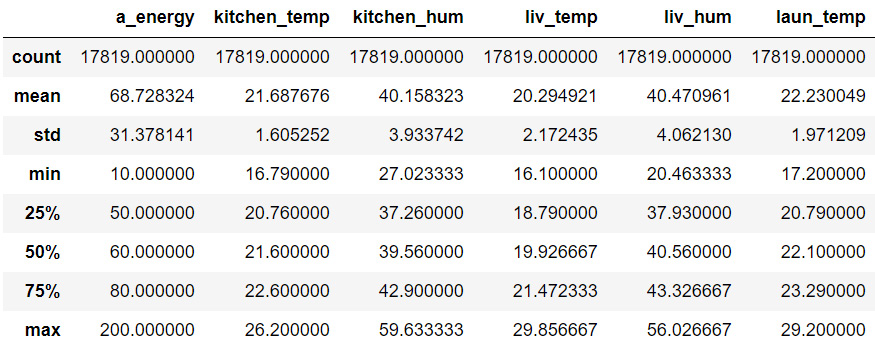
Figure 9.10: The first five rows of energy

Now the count of all the columns is 17819 because we dropped the instances in which a_energy was above 200 Wh. The maximum value in a_energy is now 200 Wh. There are 27 columns in the describe table since we dropped l_energy, and the date_time column doesn't appear here.

We have now successfully analyzed the a_energy column, removed the outliers, and prepared a new DataFrame that we will use for further analyses.

Note

The solution to the activity can be found on page 562.

Let's now move toward feature engineering to bring more efficacy into our analysis.

Exercise 9.03: Performing Feature Engineering

In this exercise, you will perform feature engineering on the date_time column of the energy DataFrame so that we can use it more efficiently to analyze the data:

1. Create a copy of the energy DataFrame and store it as new_en:

   new_en = energy

2. Convert the date_time column of new_en into the DateTime format – %Y-%m-%d %H:%M:%S – using the .to_datetime() function:

   new_en['date_time'] = pd.to_datetime(new_en.date_time,

                                        format = '%Y-%m-%d %H:%M:%S')

3. Print the first five rows of new_en:

   new_en.head()

   The output will be as follows:

   

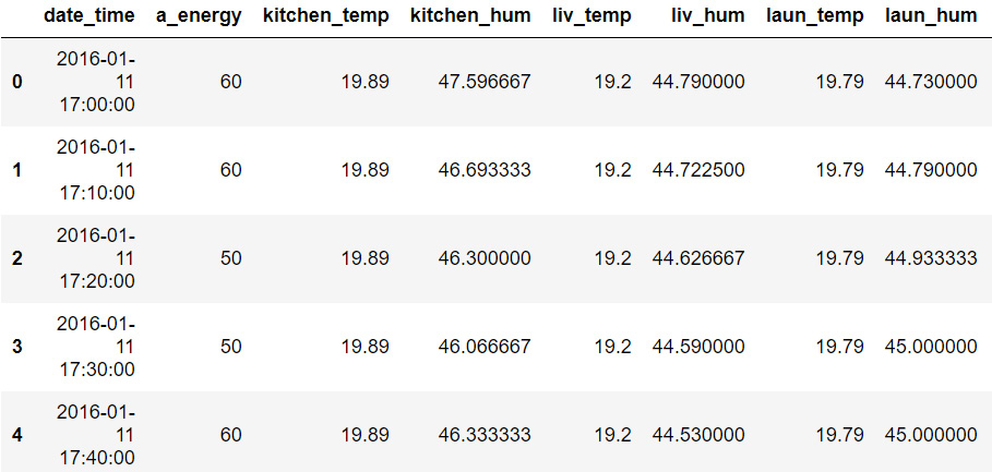
   Figure 9.11: The converted date_time column

4. Insert a column at index position 1 called month, whose value is the month from the date_time column extracted using the dt.month function:

   new_en.insert(loc = 1, column = 'month',

                 value = new_en.date_time.dt.month)

5. Insert another column at index position 2 called day, whose value is the day of the week extracted using the dt.dayofweek function. Add 1 to this value so that the numbers are between 1 and 7:

   new_en.insert(loc = 2, column = 'day',

                 value = (new_en.date_time.dt.dayofweek)+1)

6. Print the first five rows of new_en:

   new_en.head()

   The output will be as follows:

   

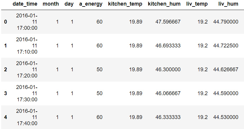
Figure 9.12: The month and day columns in new_en

Note

To access the source code for this specific section, please refer to https://packt.live/2C9Sjnz.

You can also run this example online at https://packt.live/2AAaOBv. You must execute the entire Notebook in order to get the desired result.

In this exercise, we have successfully created two new features (the month and the day of the week) from one original feature (date_time). These new features will help us conduct a detailed time series analysis and derive greater insight from our data. This method of feature engineering can be applied to other features as well. In the previous chapter, for instance, we created a feature called spent whose values were the product of values from two other features.

Let's now solve an exercise to picture the dataset, which will certainly help us to have better insights into the data.

Exercise 9.04: Visualizing the Dataset

In this exercise, you will visualize various features from the new_en DataFrame we created at the end of Exercise 9.03, Performing Feature Engineering to observe patterns and relationships. We are going to use a new Python library called plotly to create visualizations. plotly is a great library to create interactive visualizations. From plotly, we are going to be using the graph_objs module.

There are a variety of Python libraries designed for data visualization, and the decision of which one to use is most commonly based on personal preference, as in general they all possess similar methods.

1. Import plotly.graph_objs:

   import plotly.graph_objs as go

2. Create a scatter plot, with the x axis as the date_time column, mode as lines, and the y axis as the a_energy column:

   app_date = go.Scatter(x = new_en.date_time,

                         mode = "lines", y = new_en.a_energy)

3. In the layout, set the title as Appliance Energy Consumed by Date, the x-axis title as Date, and the y-axis title as Wh:

   layout = go.Layout(title = 'Appliance Energy Consumed by Date',

                      xaxis = dict(title='Date'),

                      yaxis = dict(title='Wh'))

4. Plot the figure using go.Figure, with the data as app_date and the layout as layout:

   fig = go.Figure(data = [app_date], layout = layout)

5. Use .show() to display the figure:

   fig.show()

   The output will be as follows:

   

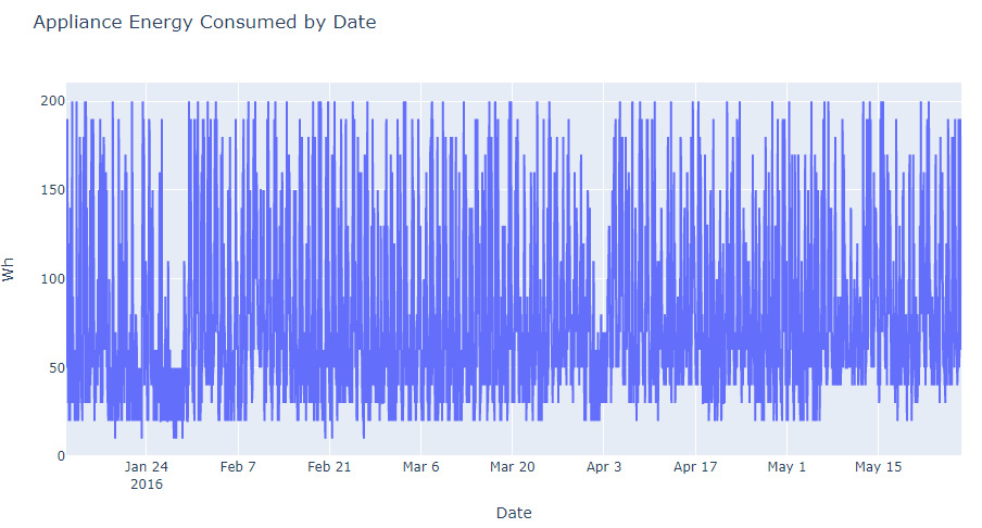
   Figure 9.13: The energy consumed by appliances per date

   The data seems quite evenly distributed; however, there is a dip in the energy consumed toward the end of January and the beginning of April. Let's take a closer look.

6. Create a table called app_month that stores the total energy consumed by appliances per month. To do this, use .groupby() on month in new_en and .sum() on a_energy. The groupby function groups a DataFrame by specific columns:

   app_mon = new_en.groupby(by = ['month'],

                            as_index = False)['a_energy'].sum()

7. Print app_mon:

   app_mon

   The output will be as follows:

   

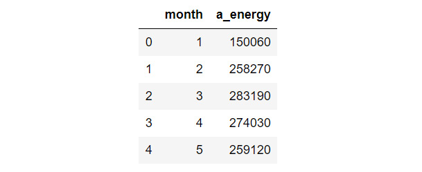
   Figure 9.14: Total energy consumed by appliances per month

8. Sort app_mon in descending order to find out which month the appliances consumed the most amount of energy:

   app_mon.sort_values(by = 'a_energy',

                       ascending = False).head()

   The output will be as follows:

   

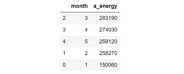
   Figure 9.15: Sorted app_mon

   As you can see, March was the month during which the appliances consumed the most energy, and it was in January that they consumed the least. The difference between the energy consumed in January and February (the month during which the second least amount of energy was consumed) is approximately 100,000 Wh itself.

9. Set the figure size as 15, 6:

   plt.subplots(figsize = (15, 6))

10. Using seaborn, create a bar plot for the month and a_energy columns in app_mon:

    am = sns.barplot(app_mon.month, app_mon.a_energy)

11. Set the x-axis label as Month, the y-axis label as Energy Consumed by Appliances, and the title as Total Energy Consumed by Appliances per Month:

    plt.xlabel('Month')

    plt.ylabel('Energy Consumed by Appliances')

    plt.title('Total Energy Consumed by Appliances per Month')

12. Display the plot using .show():

    plt.show()

    The output will be as follows:

    

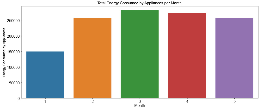
Figure 9.16: The total energy consumed by appliances per month

Note

To access the source code for this specific section, please refer to https://packt.live/2BbwHqy.

You can also run this example online at https://packt.live/3eat9DA. You must execute the entire Notebook in order to get the desired result.

This graph displays the observations we made in the app_mon table.

Activity 9.02: Observing the Trend between a_energy and day

In this activity, you are going to repeat this process with the day column, observing the relationship between a_energy and day:

1. Create a table called app_day that stores the total energy consumed by appliances per day of the week. To do this, use .groupby() on day in new_en and .sum() on a_energy.
2. Print app_day.

   The output will be as follows:

   

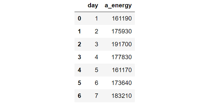
   Figure 9.17: The total energy consumed by appliances per day of the week

   As you can see in the preceding output, the days are numbered as 1, 2, and so on to represent Monday, Tuesday, and so on respectively.

3. Sort app_day in descending order to find out which day of the week the appliances consumed the most amount of energy.

   The output will be as follows:

   

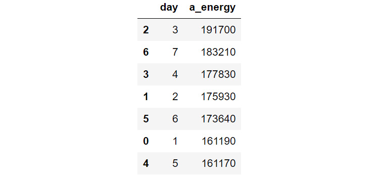
   Figure 9.18: The total energy consumed by appliances on different days of the week

   This table indicates that Wednesdays were the days when the appliances consumed the most energy, which is a bit odd. The following day in the table is Sunday, which makes sense since people might be at home more. The day the least energy was consumed was Friday.

4. Set the figure size as 15, 6.
5. Using seaborn, create a bar plot for the day and a_energy columns in app_day.
6. Set the x-axis label as Day of the Week, the y-axis label as Energy Consumed by Appliances, and the title as Total Energy Consumed by Appliances.
7. Display the plot using .show().

   The output will be as follows:

   

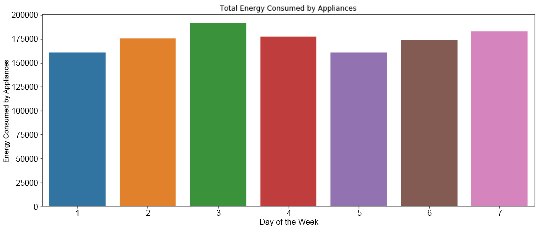
Figure 9.19: The total energy consumed by appliances each day of the week

As you can see, the greatest amount of energy is consumed on Wednesdays and the least energy is consumed on Fridays.

Note

The solution to the activity can be found on page 564.

In this activity, we successfully observed the energy consumed per day of the week. In the following exercise and activity, we are going to look into the other features more closely.

Exercise 9.05: Plotting Distributions of the Temperature Columns

In this exercise, you will plot distributions of the temperature columns to check whether any of them contain skewed data:

1. Create a list called col_temp containing all the column names from new_en that contain data regarding temperature:

   col_temp = ['kitchen_temp', 'liv_temp', 'laun_temp',

               'off_temp', 'bath_temp', 'out_b_temp',

               'iron_temp', 'teen_temp', 'par_temp']

2. Create a DataFrame called temp, containing data of the columns mentioned in col_temp:

   temp = new_en[col_temp]

3. Print the first five rows of temp:

   temp.head()

   The output will be as follows:

   

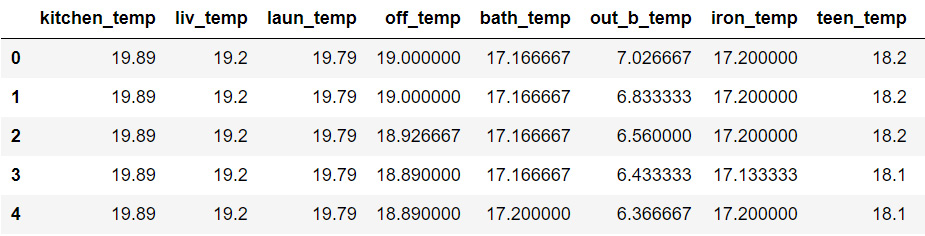
   Figure 9.20: The temp DataFrame

4. Plot a histogram for each of these temperature columns with 15 bins each:

   temp.hist(bins = 15, figsize = (12, 16))

   Since we are plotting distributions of the temperature columns, the y axis is the count and the x axis is the temperature in Celsius.

   The output will be as follows:

   

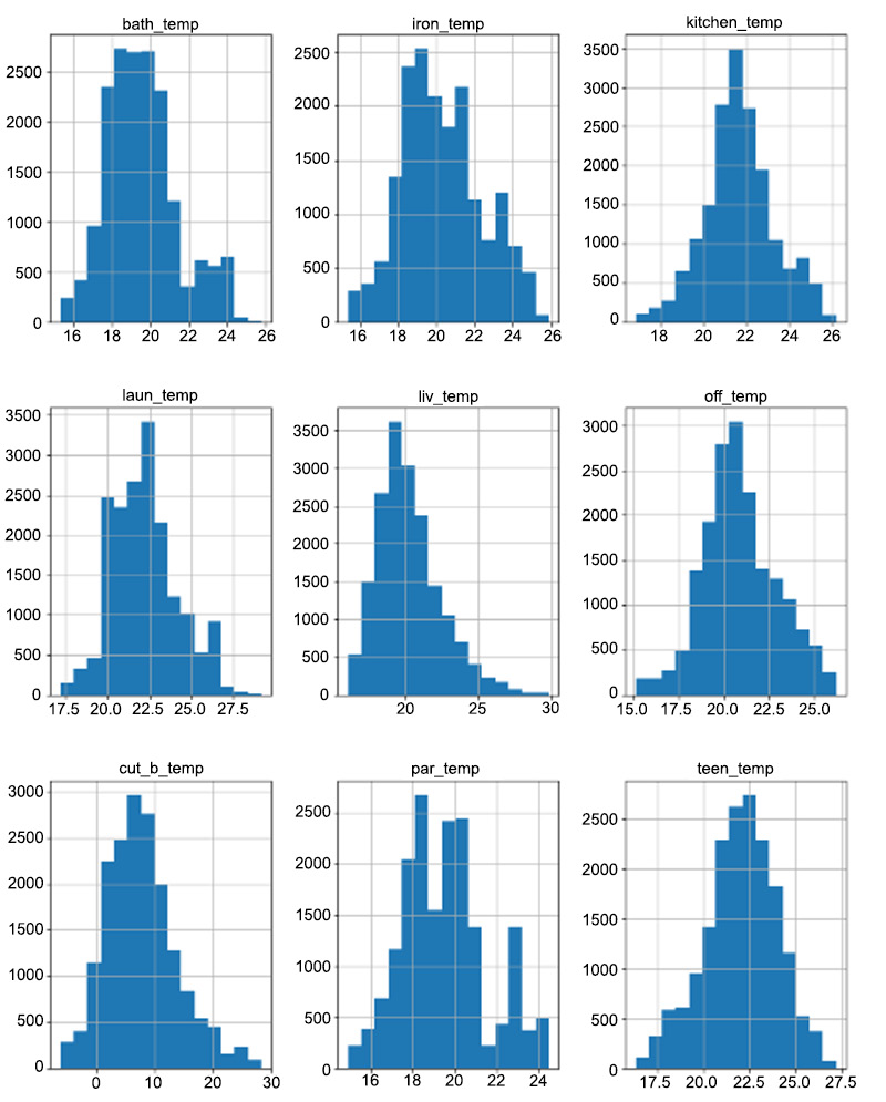
Figure 9.21: The distributions of the temperature variables

Note

To access the source code for this specific section, please refer to https://packt.live/3fA6j8P.

You can also run this example online at https://packt.live/30PqdIP. You must execute the entire Notebook in order to get the desired result.

All of these distributions seem to be following the normal distribution as they are spread across the scale with a few gradual surges in between. As you can see, there are no sudden rises or falls through the distribution and so we can conclude that the temperature data is not skewed.

Note

To find out more about the normal distribution, click here:

https://www.investopedia.com/terms/n/normaldistribution.asp

Activity 9.03: Plotting Distributions of the Humidity Columns

In this activity, you will repeat the steps of Exercise 9.05, Plotting Distributions of Temperature Columns but for the humidity columns and the external columns:

1. Create a list called col_hum, consisting of the humidity columns from new_en.
2. Create a DataFrame called hum, containing data from the columns mentioned in col_hum.
3. Print the first five rows of hum.

   The output will be as follows:

   

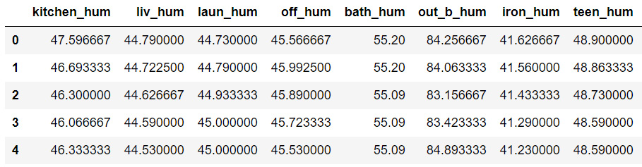
   Figure 9.22: The hum DataFrame

4. Plot a histogram for each of these variables with 15 bins each.

   Since we are plotting distributions of the humidity columns, the y axis is the count and the x axis is the humidity expressed as a percentage.

   The output will be as follows:

   

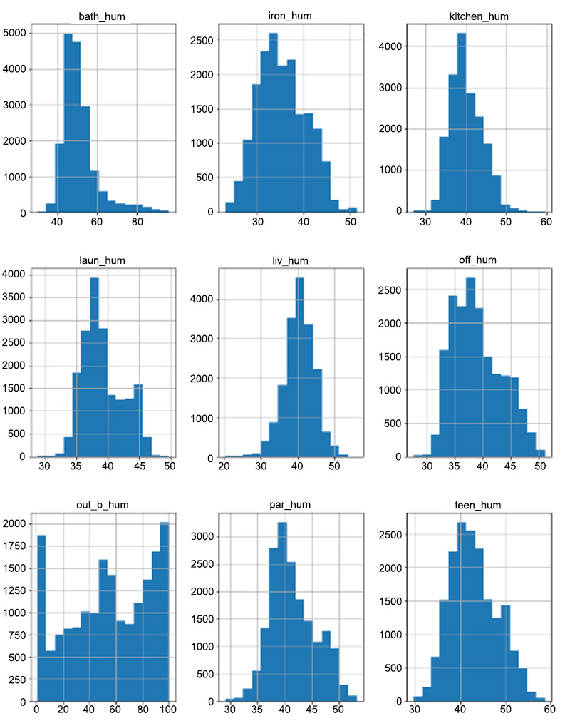
   Figure 9.23: The distributions of the humidity variables

   All the distributions except out_b_hum appear to be following the normal distribution. As you can see, the distribution of out_b_hum rises steeply at the extremes of the scale and the rest of the data points are spread unevenly across the x axis. Plot the distributions of the remaining variables first, and then take a closer look at out_b_hum.

5. Create a list called col_weather consisting of the remaining columns from new_en.
6. Create a DataFrame called weath containing data from the columns mentioned in col_weather. The first five rows of weath should be as follows:
   

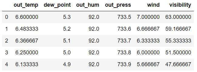
   Figure 9.24: The weath DataFrame

7. Plot a histogram for each of these variables with 15 bins each.

   Since we are plotting distributions, the y axis is the count and the x axis is the feature we are plotting. For example, the x axis in the case of wind is windspeed.

   The output should be similar to the following:

   

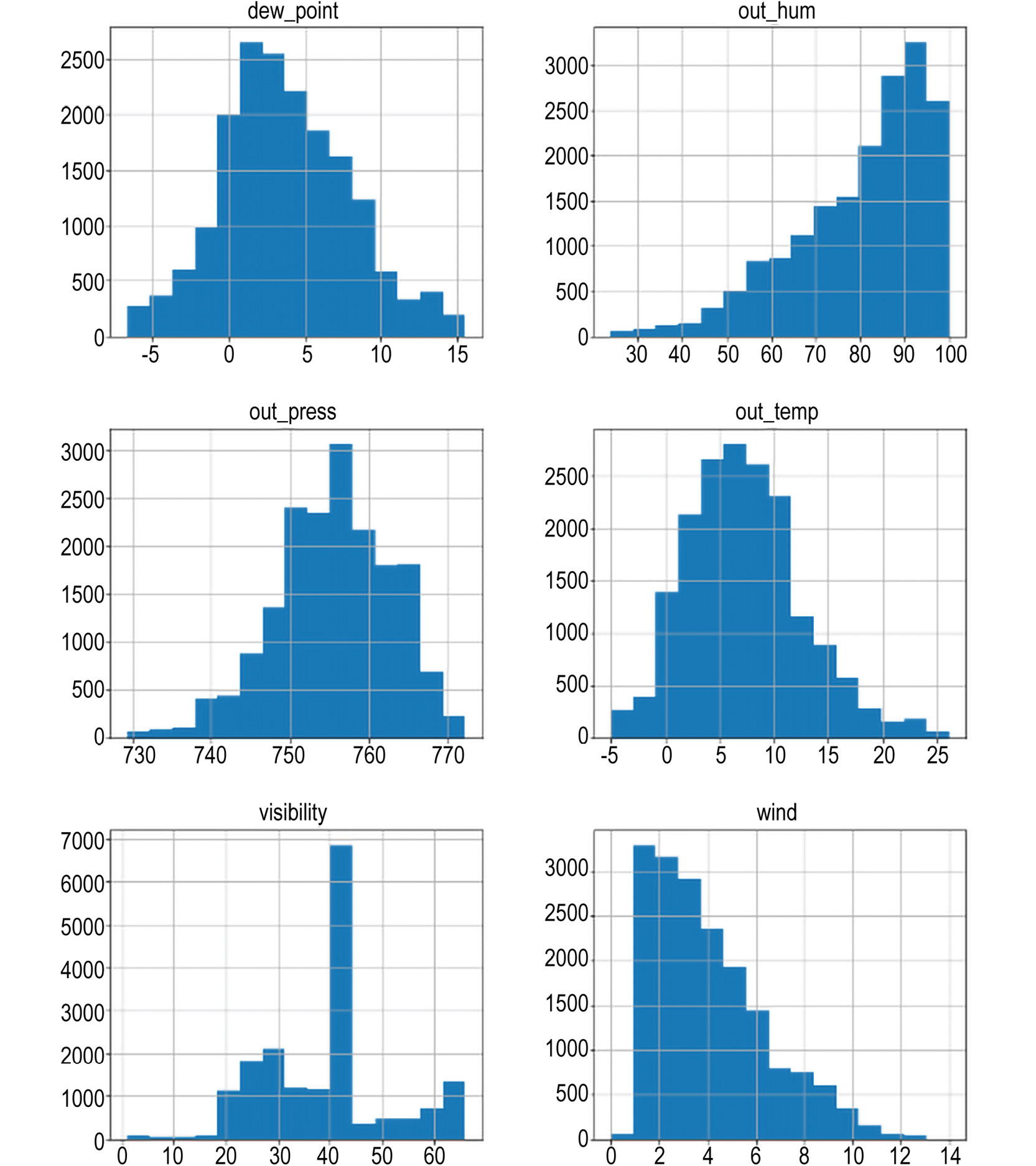
Figure 9.25: The distributions of the weather variables

Note

The solution to the activity can be found on page 567.

In this activity, we have successfully plotted the distributions of all the features from our data and determined which ones follow a normal distribution and which ones don't. As you can see, three of these distributions are not normal: out_hum, visibility, and wind, as they appear to show steep rises/falls through the plot. We need to find out the reason for this, as they will largely influence the input parameters fed to a machine learning model.

In the following exercise, we are going to take a closer look at four features that we have concluded do not seem like normal distributions. Taking a closer look at data is always beneficial since it helps us determine whether data is skewed or not, and based on that, whether those features should be used as input for machine learning models or not. Hence, this technique can be used in multiple different scenarios too, to assess the quality and distribution of your data.

Exercise 9.06: Plotting out_b, out_hum, visibility, and wind

In this exercise, you will plot the distribution for the features of out_b, out_hum, visibility, and wind to determine how important these features are so that we can decide whether they can be used as inputs for machine learning models:

1. Set the axes and figure sizes:

   f, ax = plt.subplots(2, 2, figsize = (12, 8))

2. Create a distribution plot using seaborn for each of the four variables:

   obh = sns.distplot(hum["out_b_hum"], bins = 10, ax = ax[0][0])

   oh = sns.distplot(weath["out_hum"], bins = 10, ax = ax[0][1])

   vis = sns.distplot(weath["visibility"], bins = 10, ax = ax[1][0])

   wind = sns.distplot(weath["wind"], bins = 10, ax = ax[1][1])

   The output will be as follows:

   

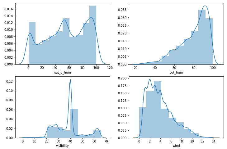
   Figure 9.26: The distribution plots for the skewed columns

   Let's plot a correlation plot to observe the relationship between all the variables.

3. Use .corr() to calculate the correlation between the variables in new_en. Save this in a variable called corr:

   corr = new_en.corr()

4. Mask the repeated values:

   mask = np.zeros_like(corr, dtype=np.bool)

   mask[np.triu_indices_from(mask)] = True

5. Set the axes and figure sizes:

   f, ax = plt.subplots(figsize=(16, 14))

6. Create a heatmap based on corr. Set the annotations as True and the number of decimal places to two, and mask as mask:

   sns.heatmap(corr, annot = True, fmt = ".2f", mask = mask)

7. Set the x- and y-axis ticks as the column names:

   plt.xticks(range(len(corr.columns)), corr.columns)

   plt.yticks(range(len(corr.columns)), corr.columns)

8. Display the plot:

   plt.show()

   The output will be as follows:

   

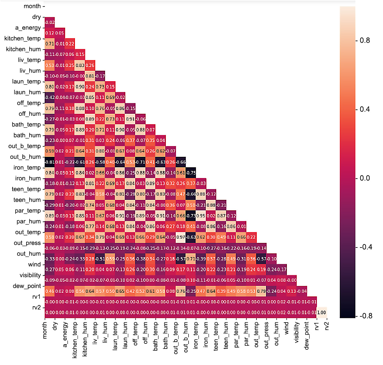
Figure 9.27: Correlation plot

Note

To access the source code for this specific section, please refer to https://packt.live/2UPoCyT.

You can also run this example online at https://packt.live/30Te719. You must execute the entire Notebook in order to get the desired result.

From this heatmap, we can see that all the temperature variables have a high positive correlation with a_energy. The outdoor weather attributes seem to have a low correlation, as well as the humidity columns. This means that the temperature has a lot to do with how much the appliances are used.

Summary

We have reached the end of this chapter and have successfully analyzed the amount of energy consumed by household appliances based on temperature, humidity, and other external weather conditions. We applied several data analysis techniques, including feature engineering and designing boxplots for specific features, to gain a better understanding of the information that the data contains. Additionally, we also plotted distributions of skewed data to observe them better.

In the next chapter, we will come to the end of our data analysis journey by applying our techniques to one last dataset. We will be analyzing and assessing the air quality of multiple localities in Beijing, China. Be ready to apply all your data analysis knowledge gained so far on this last dataset.