Chapter 3

Retail Sales

The best way to understand the principles of dimensional modeling is to work through a series of tangible examples. By visualizing real cases, you hold the particular design challenges and solutions in your mind more effectively than if they are presented abstractly. This book uses case studies from a range of businesses to help move past the idiosyncrasies of your own environment and reinforce dimensional modeling best practices.

To learn dimensional modeling, please read all the chapters in this book, even if you don't manage a retail store or work for a telecommunications company. The chapters are not intended to be full-scale solutions for a given industry or business function. Each chapter covers a set of dimensional modeling patterns that comes up in nearly every kind of business. Universities, insurance companies, banks, and airlines alike surely need the techniques developed in this retail chapter. Besides, thinking about someone else's business is refreshing. It is too easy to let historical complexities derail you when dealing with data from your company. By stepping outside your organization and then returning with a well-understood design principle (or two), it is easier to remember the spirit of the design principles as you descend into the intricate details of your business.

Chapter 3 discusses the following concepts:

• Four-step process for designing dimensional models
• Fact table granularity
• Transaction fact tables
• Additive, non-additive, and derived facts
• Dimension attributes, including indicators, numeric descriptors, and multiple hierarchies
• Calendar date dimensions, plus time-of-day
• Causal dimensions, such as promotion
• Degenerate dimensions, such as the transaction receipt number
• Nulls in a dimensional model
• Extensibility of dimension models
• Factless fact tables
• Surrogate, natural, and durable keys
• Snowflaked dimension attributes
• Centipede fact tables with “too many dimensions”

Four-Step Dimensional Design Process

Throughout this book, we will approach the design of a dimensional model by consistently considering four steps, as the following sections discuss in more detail.

Step 1: Select the Business Process

A business process is a low-level activity performed by an organization, such as taking orders, invoicing, receiving payments, handling service calls, registering students, performing a medical procedure, or processing claims. To identify your organization's business processes, it's helpful to understand several common characteristics:

• Business processes are frequently expressed as action verbs because they represent activities that the business performs. The companion dimensions describe descriptive context associated with each business process event.
• Business processes are typically supported by an operational system, such as the billing or purchasing system.
• Business processes generate or capture key performance metrics. Sometimes the metrics are a direct result of the business process; the measurements are derivations at other times. Analysts invariably want to scrutinize and evaluate these metrics by a seemingly limitless combination of filters and constraints.
• Business processes are usually triggered by an input and result in output metrics. In many organizations, there's a series of processes in which the outputs from one process become the inputs to the next. In the parlance of a dimensional modeler, this series of processes results in a series of fact tables.

You need to listen carefully to the business to identify the organization's business processes because business users can't readily answer the question, “What business process are you interested in?” The performance measurements users want to analyze in the DW/BI system result from business process events.

Sometimes business users talk about strategic business initiatives instead of business processes. These initiatives are typically broad enterprise plans championed by executive leadership to deliver competitive advantage. In order to tie a business initiative to a business process representing a project-sized unit of work for the DW/BI team, you need to decompose the business initiative into the underlying processes. This means digging a bit deeper to understand the data and operational systems that support the initiative's analytic requirements.

It's also worth noting what a business process is not. Organizational business departments or functions do not equate to business processes. By focusing on processes, rather than on functional departments, consistent information is delivered more economically throughout the organization. If you design departmentally bound dimensional models, you inevitably duplicate data with different labels and data values. The best way to ensure consistency is to publish the data once.

Step 2: Declare the Grain

Declaring the grain means specifying exactly what an individual fact table row represents. The grain conveys the level of detail associated with the fact table measurements. It provides the answer to the question, “How do you describe a single row in the fact table?” The grain is determined by the physical realities of the operational system that captures the business process's events.

Example grain declarations include:

• One row per scan of an individual product on a customer's sales transaction
• One row per line item on a bill from a doctor
• One row per individual boarding pass scanned at an airport gate
• One row per daily snapshot of the inventory levels for each item in a warehouse
• One row per bank account each month

These grain declarations are expressed in business terms. Perhaps you were expecting the grain to be a traditional declaration of the fact table's primary key. Although the grain ultimately is equivalent to the primary key, it's a mistake to list a set of dimensions and then assume this list is the grain declaration. Whenever possible, you should express the grain in business terms.

Dimensional modelers sometimes try to bypass this seemingly unnecessary step of the four-step design process. Please don't! Declaring the grain is a critical step that can't be taken lightly. In debugging thousands of dimensional designs over the years, the most frequent error is not declaring the grain of the fact table at the beginning of the design process. If the grain isn't clearly defined, the whole design rests on quicksand; discussions about candidate dimensions go around in circles, and rogue facts sneak into the design. An inappropriate grain haunts a DW/BI implementation! It is extremely important that everyone on the design team reaches agreement on the fact table's granularity. Having said this, you may discover in steps 3 or 4 of the design process that the grain statement is wrong. This is okay, but then you must return to step 2, restate the grain correctly, and revisit steps 3 and 4 again.

Step 3: Identify the Dimensions

Dimensions fall out of the question, “How do business people describe the data resulting from the business process measurement events?” You need to decorate fact tables with a robust set of dimensions representing all possible descriptions that take on single values in the context of each measurement. If you are clear about the grain, the dimensions typically can easily be identified as they represent the “who, what, where, when, why, and how” associated with the event. Examples of common dimensions include date, product, customer, employee, and facility. With the choice of each dimension, you then list all the discrete, text-like attributes that flesh out each dimension table.

Step 4: Identify the Facts

Facts are determined by answering the question, “What is the process measuring?” Business users are keenly interested in analyzing these performance metrics. All candidate facts in a design must be true to the grain defined in step 2. Facts that clearly belong to a different grain must be in a separate fact table. Typical facts are numeric additive figures, such as quantity ordered or dollar cost amount.

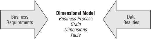
You need to consider both your business users' requirements and the realities of your source data in tandem to make decisions regarding the four steps, as illustrated in Figure 3.1. We strongly encourage you to resist the temptation to model the data by looking at source data alone. It may be less intimidating to dive into the data rather than interview a business person; however, the data is no substitute for business user input. Unfortunately, many organizations have attempted this path-of-least-resistance data-driven approach but without much success.

Figure 3.1 Key input to the four-step dimensional design process.

Retail Case Study

Let's start with a brief description of the retail business used in this case study. We begin with this industry simply because it is one we are all familiar with. But the patterns discussed in the context of this case study are relevant to virtually every dimensional model regardless of the industry.

Imagine you work in the headquarters of a large grocery chain. The business has 100 grocery stores spread across five states. Each store has a full complement of departments, including grocery, frozen foods, dairy, meat, produce, bakery, floral, and health/beauty aids. Each store has approximately 60,000 individual products, called stock keeping units (SKUs), on its shelves.

Data is collected at several interesting places in a grocery store. Some of the most useful data is collected at the cash registers as customers purchase products. The point-of-sale (POS) system scans product barcodes at the cash register, measuring consumer takeaway at the front door of the grocery store, as illustrated in Figure 3.2's cash register receipt. Other data is captured at the store's back door where vendors make deliveries.

Figure 3.2 Sample cash register receipt.

At the grocery store, management is concerned with the logistics of ordering, stocking, and selling products while maximizing profit. The profit ultimately comes from charging as much as possible for each product, lowering costs for product acquisition and overhead, and at the same time attracting as many customers as possible in a highly competitive environment. Some of the most significant management decisions have to do with pricing and promotions. Both store management and headquarters marketing spend a great deal of time tinkering with pricing and promotions. Promotions in a grocery store include temporary price reductions, ads in newspapers and newspaper inserts, displays in the grocery store, and coupons. The most direct and effective way to create a surge in the volume of product sold is to lower the price dramatically. A 50-cent reduction in the price of paper towels, especially when coupled with an ad and display, can cause the sale of the paper towels to jump by a factor of 10. Unfortunately, such a big price reduction usually is not sustainable because the towels probably are being sold at a loss. As a result of these issues, the visibility of all forms of promotion is an important part of analyzing the operations of a grocery store.

Now that we have described our business case study, we'll begin to design the dimensional model.

Step 1: Select the Business Process

The first step in the design is to decide what business process to model by combining an understanding of the business requirements with an understanding of the available source data.

In our retail case study, management wants to better understand customer purchases as captured by the POS system. Thus the business process you're modeling is POS retail sales transactions. This data enables the business users to analyze which products are selling in which stores on which days under what promotional conditions in which transactions.

Step 2: Declare the Grain

After the business process has been identified, the design team faces a serious decision about the granularity. What level of data detail should be made available in the dimensional model?

Tackling data at its lowest atomic grain makes sense for many reasons. Atomic data is highly dimensional. The more detailed and atomic the fact measurement, the more things you know for sure. All those things you know for sure translate into dimensions. In this regard, atomic data is a perfect match for the dimensional approach.

Atomic data provides maximum analytic flexibility because it can be constrained and rolled up in every way possible. Detailed data in a dimensional model is poised and ready for the ad hoc attack by business users.

Of course, you could declare a more summarized granularity representing an aggregation of the atomic data. However, as soon as you select a higher level grain, you limit yourself to fewer and/or potentially less detailed dimensions. The less granular model is immediately vulnerable to unexpected user requests to drill down into the details. Users inevitably run into an analytic wall when not given access to the atomic data. Although aggregated data plays an important role for performance tuning, it is not a substitute for giving users access to the lowest level details; users can easily summarize atomic data, but it's impossible to create details from summary data. Unfortunately, some industry pundits remain confused about this point. They claim dimensional models are only appropriate for summarized data and then criticize the dimensional modeling approach for its supposed need to anticipate the business question. This misunderstanding goes away when detailed, atomic data is made available in a dimensional model.

In our case study, the most granular data is an individual product on a POS transaction, assuming the POS system rolls up all sales for a given product within a shopping cart into a single line item. Although users probably are not interested in analyzing single items associated with a specific POS transaction, you can't predict all the ways they'll want to cull through that data. For example, they may want to understand the difference in sales on Monday versus Sunday. Or they may want to assess whether it's worthwhile to stock so many individual sizes of certain brands. Or they may want to understand how many shoppers took advantage of the 50-cents-off promotion on shampoo. Or they may want to determine the impact of decreased sales when a competitive diet soda product was promoted heavily. Although none of these queries calls for data from one specific transaction, they are broad questions that require detailed data sliced in precise ways. None of them could have been answered if you elected to provide access only to summarized data.

Step 3: Identify the Dimensions

After the grain of the fact table has been chosen, the choice of dimensions is straightforward. The product and transaction fall out immediately. Within the framework of the primary dimensions, you can ask whether other dimensions can be attributed to the POS measurements, such as the date of the sale, the store where the sale occurred, the promotion under which the product is sold, the cashier who handled the sale, and potentially the method of payment. We express this as another design principle.

The following descriptive dimensions apply to the case: date, product, store, promotion, cashier, and method of payment. In addition, the POS transaction ticket number is included as a special dimension, as described in the section “Degenerate Dimensions for Transaction Numbers” later in this chapter.

Before fleshing out the dimension tables with descriptive attributes, let's complete the final step of the four-step process. You don't want to lose sight of the forest for the trees at this stage of the design.

Step 4: Identify the Facts

The fourth and final step in the design is to make a careful determination of which facts will appear in the fact table. Again, the grain declaration helps anchor your thinking. Simply put, the facts must be true to the grain: the individual product line item on the POS transaction in this case. When considering potential facts, you may again discover adjustments need to be made to either your earlier grain assumptions or choice of dimensions.

The facts collected by the POS system include the sales quantity (for example, the number of cans of chicken noodle soup), per unit regular, discount, and net paid prices, and extended discount and sales dollar amounts. The extended sales dollar amount equals the sales quantity multiplied by the net unit price. Likewise, the extended discount dollar amount is the sales quantity multiplied by the unit discount amount. Some sophisticated POS systems also provide a standard dollar cost for the product as delivered to the store by the vendor. Presuming this cost fact is readily available and doesn't require a heroic activity-based costing initiative, you can include the extended cost amount in the fact table. The fact table begins to take shape in Figure 3.3.

Figure 3.3 Measured facts in retail sales schema.

Four of the facts, sales quantity and the extended discount, sales, and cost dollar amounts, are beautifully additive across all the dimensions. You can slice and dice the fact table by the dimension attributes with impunity, and every sum of these four facts is valid and correct.

Derived Facts

You can compute the gross profit by subtracting the extended cost dollar amount from the extended sales dollar amount, or revenue. Although computed, gross profit is also perfectly additive across all the dimensions; you can calculate the gross profit of any combination of products sold in any set of stores on any set of days. Dimensional modelers sometimes question whether a calculated derived fact should be stored in the database. We generally recommend it be stored physically. In this case study, the gross profit calculation is straightforward, but storing it means it's computed consistently in the ETL process, eliminating the possibility of user calculation errors. The cost of a user incorrectly representing gross profit overwhelms the minor incremental storage cost. Storing it also ensures all users and BI reporting applications refer to gross profit consistently. Because gross profit can be calculated from adjacent data within a single fact table row, some would argue that you should perform the calculation in a view that is indistinguishable from the table. This is a reasonable approach if all users access the data via the view and no users with ad hoc query tools can sneak around the view to get at the physical table. Views are a reasonable way to minimize user error while saving on storage, but the DBA must allow no exceptions to accessing the data through the view. Likewise, some organizations want to perform the calculation in the BI tool. Again, this works if all users access the data using a common tool, which is seldom the case in our experience. However, sometimes non-additive metrics on a report such as percentages or ratios must be computed in the BI application because the calculation cannot be precalculated and stored in a fact table. OLAP cubes excel in these situations.

Non-Additive Facts

Gross margin can be calculated by dividing the gross profit by the extended sales dollar revenue. Gross margin is a non-additive fact because it can't be summarized along any dimension. You can calculate the gross margin of any set of products, stores, or days by remembering to sum the revenues and costs respectively before dividing.

Unit price is another non-additive fact. Unlike the extended amounts in the fact table, summing unit price across any of the dimensions results in a meaningless, nonsensical number. Consider this simple example: You sold one widget at a unit price of $1.00 and four widgets at a unit price of 50 cents each. You could sum the sales quantity to determine that five widgets were sold. Likewise, you could sum the sales dollar amounts ($1.00 and $2.00) to arrive at a total sales amount of $3.00. However, you can't sum the unit prices ($1.00 and 50 cents) and declare that the total unit price is $1.50. Similarly, you shouldn't announce that the average unit price is 75 cents. The properly weighted average unit price should be calculated by taking the total sales amount ($3.00) and dividing by the total quantity (five widgets) to arrive at a 60 cent average unit price. You'd never arrive at this conclusion by looking at the unit price for each transaction line in isolation. To analyze the average price, you must add up the sales dollars and sales quantities before dividing the total dollars by the total quantity sold. Fortunately, many BI tools perform this function correctly. Some question whether non-additive facts should be physically stored in a fact table. This is a legitimate question given their limited analytic value, aside from printing individual values on a report or applying a filter directly on the fact, which are both atypical. In some situations, a fundamentally non-additive fact such as a temperature is supplied by the source system. These non-additive facts may be averaged carefully over many records, if the business analysts agree that this makes sense.

Transaction Fact Tables

Transactional business processes are the most common. The fact tables representing these processes share several characteristics:

• The grain of atomic transaction fact tables can be succinctly expressed in the context of the transaction, such as one row per transaction or one row per transaction line.
• Because these fact tables record a transactional event, they are often sparsely populated. In our case study, we certainly wouldn't sell every product in every shopping cart.
• Even though transaction fact tables are unpredictably and sparsely populated, they can be truly enormous. Most billion and trillion row tables in a data warehouse are transaction fact tables.
• Transaction fact tables tend to be highly dimensional.
• The metrics resulting from transactional events are typically additive as long as they have been extended by the quantity amount, rather than capturing per unit metrics.

At this early stage of the design, it is often helpful to estimate the number of rows in your largest table, the fact table. In this case study, it simply may be a matter of talking with a source system expert to understand how many POS transaction line items are generated on a periodic basis. Retail traffic fluctuates significantly from day to day, so you need to understand the transaction activity over a reasonable period of time. Alternatively, you could estimate the number of rows added to the fact table annually by dividing the chain's annual gross revenue by the average item selling price. Assuming that gross revenues are $4 billion per year and that the average price of an item on a customer ticket is $2.00, you can calculate that there are approximately 2 billion transaction line items per year. This is a typical engineer's estimate that gets you surprisingly close to sizing a design directly from your armchair. As designers, you always should be triangulating to determine whether your calculations are reasonable.

Dimension Table Details

Now that we've walked through the four-step process, let's return to the dimension tables and focus on populating them with robust attributes.

Date Dimension

The date dimension is a special dimension because it is the one dimension nearly guaranteed to be in every dimensional model since virtually every business process captures a time series of performance metrics. In fact, date is usually the first dimension in the underlying partitioning scheme of the database so that the successive time interval data loads are placed into virgin territory on the disk.

For readers of the first edition of The Data Warehouse Toolkit (Wiley, 1996), this dimension was referred to as the time dimension. However, for more than a decade, we've used the “date dimension” to mean a daily grained dimension table. This helps distinguish between date and time-of-day dimensions.

Unlike most of the other dimensions, you can build the date dimension table in advance. You may put 10 or 20 years of rows representing individual days in the table, so you can cover the history you have stored, as well as several years in the future. Even 20 years' worth of days is only approximately 7,300 rows, which is a relatively small dimension table. For a daily date dimension table in a retail environment, we recommend the partial list of columns shown in Figure 3.4.

Figure 3.4 Date dimension table.

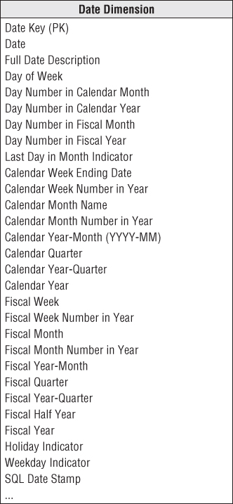
Each column in the date dimension table is defined by the particular day that the row represents. The day-of-week column contains the day's name, such as Monday. This column would be used to create reports comparing Monday business with Sunday business. The day number in calendar month column starts with 1 at the beginning of each month and runs to 28, 29, 30, or 31 depending on the month. This column is useful for comparing the same day each month. Similarly, you could have a month number in year (1, …, 12). All these integers support simple date arithmetic across year and month boundaries.

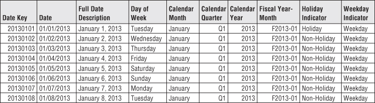
For reporting, you should include both long and abbreviated labels. For example, you would want a month name attribute with values such as January. In addition, a year-month (YYYY-MM) column is useful as a report column header. You likely also want a quarter number (Q1, …, Q4), as well as a year-quarter, such as 2013-Q1. You would include similar columns for the fiscal periods if they differ from calendar periods. Sample rows containing several date dimension columns are illustrated in Figure 3.5.

Figure 3.5 Date dimension sample rows.

Some designers pause at this point to ask why an explicit date dimension table is needed. They reason that if the date key in the fact table is a date type column, then any SQL query can directly constrain on the fact table date key and use natural SQL date semantics to filter on month or year while avoiding a supposedly expensive join. This reasoning falls apart for several reasons. First, if your relational database can't handle an efficient join to the date dimension table, you're in deep trouble. Most database optimizers are quite efficient at resolving dimensional queries; it is not necessary to avoid joins like the plague.

Since the average business user is not versed in SQL date semantics, he would be unable to request typical calendar groupings. SQL date functions do not support filtering by attributes such as weekdays versus weekends, holidays, fiscal periods, or seasons. Presuming the business needs to slice data by these nonstandard date attributes, then an explicit date dimension table is essential. Calendar logic belongs in a dimension table, not in the application code.

Flags and Indicators as Textual Attributes

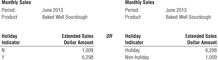
Like many operational flags and indicators, the date dimension's holiday indicator is a simple indicator with two potential values. Because dimension table attributes serve as report labels and values in pull-down query filter lists, this indicator should be populated with meaningful values such as Holiday or Non-holiday instead of the cryptic Y/N, 1/0, or True/False. As illustrated in Figure 3.6, imagine a report comparing holiday versus non-holiday sales for a product. More meaningful domain values for this indicator translate into a more meaningful, self-explanatory report. Rather than decoding flags into understandable labels in the BI application, we prefer that decoded values be stored in the database so they're consistently available to all users regardless of their BI reporting environment or tools.

Figure 3.6 Sample reports with cryptic versus textual indicators.

A similar argument holds true for the weekday indicator that would have a value of Weekday or Weekend. Saturdays and Sundays obviously would be assigned the weekend value. Of course, multiple date table attributes can be jointly constrained, so you can easily compare weekday holidays with weekend holidays.

Current and Relative Date Attributes

Most date dimension attributes are not subject to updates. June 1, 2013 will always roll up to June, Calendar Q2, and 2013. However, there are attributes you can add to the basic date dimension that will change over time, including IsCurrentDay, IsCurrentMonth, IsPrior60Days, and so on. IsCurrentDay obviously must be updated each day; the attribute is useful for generating reports that always run for today. A nuance to consider is the day that IsCurrentDay refers to. Most data warehouses load data daily, so IsCurrentDay would refer to yesterday (or more accurately, the most recent day loaded). You might also add attributes to the date dimension that are unique to your corporate calendar, such as IsFiscalMonthEnd.

Some date dimensions include updated lag attributes. The lag day column would take the value 0 for today, –1 for yesterday, +1 for tomorrow, and so on. This attribute could easily be a computed column rather than physically stored. It might be useful to set up similar structures for month, quarter, and year. Many BI tools include functionality to do prior period calculations, so these lag columns may be unnecessary.

Time-of-Day as a Dimension or Fact

Although date and time are comingled in an operational date/time stamp, time-of-day is typically separated from the date dimension to avoid a row count explosion in the date dimension. As noted earlier, a date dimension with 20 years of history contains approximately 7,300 rows. If you changed the grain of this dimension to one row per minute in a day, you'd end up with over 10 million rows to accommodate the 1,440 minutes per day. If you tracked time to the second, you'd have more than 31 million rows per year! Because the date dimension is likely the most frequently constrained dimension in a schema, it should be kept as small and manageable as possible.

If you want to filter or roll up time periods based on summarized day part groupings, such as activity during 15-minute intervals, hours, shifts, lunch hour, or prime time, time-of-day would be treated as a full-fledged dimension table with one row per discrete time period, such as one row per minute within a 24-hour period resulting in a dimension with 1,440 rows.

If there's no need to roll up or filter on time-of-day groupings, time-of-day should be handled as a simple date/time fact in the fact table. By the way, business users are often more interested in time lags, such as the transaction's duration, rather than discreet start and stop times. Time lags can easily be computed by taking the difference between date/time stamps. These date/time stamps also allow an application to determine the time gap between two transactions of interest, even if these transactions exist in different days, months, or years.

Product Dimension

The product dimension describes every SKU in the grocery store. Although a typical store may stock 60,000 SKUs, when you account for different merchandising schemes and historical products that are no longer available, the product dimension may have 300,000 or more rows. The product dimension is almost always sourced from the operational product master file. Most retailers administer their product master file at headquarters and download a subset to each store's POS system at frequent intervals. It is headquarters' responsibility to define the appropriate product master record (and unique SKU number) for each new product.

Flatten Many-to-One Hierarchies

The product dimension represents the many descriptive attributes of each SKU. The merchandise hierarchy is an important group of attributes. Typically, individual SKUs roll up to brands, brands roll up to categories, and categories roll up to departments. Each of these is a many-to-one relationship. This merchandise hierarchy and additional attributes are shown for a subset of products in Figure 3.7.

Figure 3.7 Product dimension sample rows.

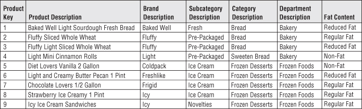
For each SKU, all levels of the merchandise hierarchy are well defined. Some attributes, such as the SKU description, are unique. In this case, there are 300,000 different values in the SKU description column. At the other extreme, there are only perhaps 50 distinct values of the department attribute. Thus, on average, there are 6,000 repetitions of each unique value in the department attribute. This is perfectly acceptable! You do not need to separate these repeated values into a second normalized table to save space. Remember dimension table space requirements pale in comparison with fact table space considerations.

Many of the attributes in the product dimension table are not part of the merchandise hierarchy. The package type attribute might have values such as Bottle, Bag, Box, or Can. Any SKU in any department could have one of these values.It often makes sense to combine a constraint on this attribute with a constraint on a merchandise hierarchy attribute. For example, you could look at all the SKUs in the Cereal category packaged in Bags. Put another way, you can browse among dimension attributes regardless of whether they belong to the merchandise hierarchy. Product dimension tables typically have more than one explicit hierarchy.

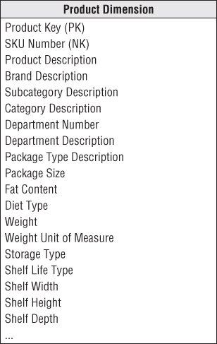
A recommended partial product dimension for a retail grocery dimensional model is shown in Figure 3.8.

Figure 3.8 Product dimension table.

Attributes with Embedded Meaning

Often operational product codes, identified in the dimension table by the NK notation for natural key, have embedded meaning with different parts of the code representing significant characteristics of the product. In this case, the multipart attribute should be both preserved in its entirety within the dimension table, as well as broken down into its component parts, which are handled as separate attributes. For example, if the fifth through ninth characters in the operational code identify the manufacturer, the manufacturer's name should also be included as a dimension table attribute.

Numeric Values as Attributes or Facts

You will sometimes encounter numeric values that don't clearly fall into either the fact or dimension attribute categories. A classic example is the standard list price for a product. It's definitely a numeric value, so the initial instinct is to place it in the fact table. But typically the standard price changes infrequently, unlike most facts that are often differently valued on every measurement event.

If the numeric value is used primarily for calculation purposes, it likely belongs in the fact table. Because standard price is non-additive, you might multiply it by the quantity for an extended amount which would be additive. Alternatively, if the standard price is used primarily for price variance analysis, perhaps the variance metric should be stored in the fact table instead. If the stable numeric value is used predominantly for filtering and grouping, it should be treated as a product dimension attribute.

Sometimes numeric values serve both calculation and filtering/grouping functions. In these cases, you should store the value in both the fact and dimension tables. Perhaps the standard price in the fact table represents the valuation at the time of the sales transaction, whereas the dimension attribute is labeled to indicate it's the current standard price.

Drilling Down on Dimension Attributes

A reasonable product dimension table can have 50 or more descriptive attributes. Each attribute is a rich source for constraining and constructing row header labels. Drilling down is nothing more than asking for a row header from a dimension that provides more information.

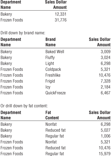
Let's say you have a simple report summarizing the sales dollar amount by department. As illustrated in Figure 3.9, if you want to drill down, you can drag any other attribute, such as brand, from the product dimension into the report next to department, and you can automatically drill down to this next level of detail. You could drill down by the fat content attribute, even though it isn't in the merchandise hierarchy rollup.

Figure 3.9 Drilling down on dimension attributes.

The product dimension is a common dimension in many dimensional models. Great care should be taken to fill this dimension with as many descriptive attributes as possible. A robust and complete set of dimension attributes translates into robust and complete analysis capabilities for the business users. We'll further explore the product dimension in Chapter 5: Procurement where we'll also discuss the handling of product attribute changes.

Store Dimension

The store dimension describes every store in the grocery chain. Unlike the product master file that is almost guaranteed to be available in every large grocery business, there may not be a comprehensive store master file. POS systems may simply supply a store number on the transaction records. In these cases, project teams must assemble the necessary components of the store dimension from multiple operational sources. Often there will be a store real estate department at headquarters who will help define a detailed store master file.

Multiple Hierarchies in Dimension Tables

The store dimension is the case study's primary geographic dimension. Each store can be thought of as a location. You can roll stores up to any geographic attribute, such as ZIP code, county, and state in the United States. Contrary to popular belief, cities and states within the United States are not a hierarchy. Since many states have identically named cities, you'll want to include a City-State attribute in the store dimension.

Stores likely also roll up an internal organization hierarchy consisting of store districts and regions. These two different store hierarchies are both easily represented in the dimension because both the geographic and organizational hierarchies are well defined for a single store row.

A recommended retail store dimension table is shown in Figure 3.10.

Figure 3.10 Store dimension table.

The floor plan type, photo processing type, and finance services type are all short text descriptors that describe the particular store. These should not be one-character codes but rather should be 10- to 20-character descriptors that make sense when viewed in a pull-down filter list or used as a report label.

The column describing selling square footage is numeric and theoretically additive across stores. You might be tempted to place it in the fact table. However, it is clearly a constant attribute of a store and is used as a constraint or label more often than it is used as an additive element in a summation. For these reasons, selling square footage belongs in the store dimension table.

Dates Within Dimension Tables

The first open date and last remodel date in the store dimension could be date type columns. However, if users want to group and constrain on nonstandard calendar attributes (like the open date's fiscal period), then they are typically join keys to copies of the date dimension table. These date dimension copies are declared in SQL by the view construct and are semantically distinct from the primary date dimension. The view declaration would look like the following:

create view first_open_date (first_open_day_number, first_open_month, …)
    as select day_number, month, …
    from date

Now the system acts as if there is another physical copy of the date dimension table called FIRST_OPEN_DATE. Constraints on this new date table have nothing to do with constraints on the primary date dimension joined to the fact table. The first open date view is a permissible outrigger to the store dimension; outriggers will be described in more detail later in this chapter. Notice we have carefully relabeled all the columns in the view so they cannot be confused with columns from the primary date dimension. These distinct logical views on a single physical date dimension are an example of dimension role playing, which we'll discuss more fully in Chapter 6: Order Management.

Promotion Dimension

The promotion dimension is potentially the most interesting dimension in the retail sales schema. The promotion dimension describes the promotion conditions under which a product is sold. Promotion conditions include temporary price reductions, end aisle displays, newspaper ads, and coupons. This dimension is often called a causal dimension because it describes factors thought to cause a change in product sales.

Business analysts at both headquarters and the stores are interested in determining whether a promotion is effective. Promotions are judged on one or more of the following factors:

• Whether the products under promotion experienced a gain in sales, called lift, during the promotional period. The lift can be measured only if the store can agree on what the baseline sales of the promoted products would have been without the promotion. Baseline values can be estimated from prior sales history and, in some cases, with the help of sophisticated models.
• Whether the products under promotion showed a drop in sales just prior to or after the promotion, canceling the gain in sales during the promotion (time shifting). In other words, did you transfer sales from regularly priced products to temporarily reduced priced products?
• Whether the products under promotion showed a gain in sales but other products nearby on the shelf showed a corresponding sales decrease (cannibalization).
• Whether all the products in the promoted category of products experienced a net overall gain in sales taking into account the time periods before, during, and after the promotion (market growth).
• Whether the promotion was profitable. Usually the profit of a promotion is taken to be the incremental gain in profit of the promoted category over the baseline sales taking into account time shifting and cannibalization, as well as the costs of the promotion.

The causal conditions potentially affecting a sale are not necessarily tracked directly by the POS system. The transaction system keeps track of price reductions and markdowns. The presence of coupons also typically is captured withthe transaction because the customer either presents coupons at the time of sale or does not. Ads and in-store display conditions may need to be linked from other sources.

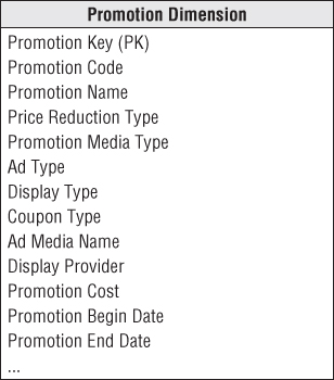
The various possible causal conditions are highly correlated. A temporary price reduction usually is associated with an ad and perhaps an end aisle display. For this reason, it makes sense to create one row in the promotion dimension for each combination of promotion conditions that occurs. Over the course of a year, there may be 1,000 ads, 5,000 temporary price reductions, and 1,000 end aisle displays, but there may be only 10,000 combinations of these three conditions affecting any particular product. For example, in a given promotion, most of the stores would run all three promotion mechanisms simultaneously, but a few of the stores may not deploy the end aisle displays. In this case, two separate promotion condition rows would be needed, one for the normal price reduction plus ad plus display and one for the price reduction plus ad only. A recommended promotion dimension table is shown in Figure 3.11.

Figure 3.11 Promotion dimension table.

From a purely logical point of view, you could record similar information about the promotions by separating the four causal mechanisms (price reductions, ads, displays, and coupons) into separate dimensions rather than combining them into one dimension. Ultimately, this choice is the designer's prerogative. The trade-offs in favor of keeping the four dimensions together include the following:

• If the four causal mechanisms are highly correlated, the combined single dimension is not much larger than any one of the separated dimensions would be.
• The combined single dimension can be browsed efficiently to see how the various price reductions, ads, displays, and coupons are used together. However, this browsing only shows the possible promotion combinations. Browsing in the dimension table does not reveal which stores or products were affected by the promotion; this information is found in the fact table.

The trade-offs in favor of separating the causal mechanisms into four distinct dimension tables include the following:

• The separated dimensions may be more understandable to the business community if users think of these mechanisms separately. This would be revealed during the business requirement interviews.
• Administration of the separate dimensions may be more straightforward than administering a combined dimension.

Keep in mind there is no difference in the content between these two choices.

Null Foreign Keys, Attributes, and Facts

Typically, many sales transactions include products that are not being promoted. Hopefully, consumers aren't just filling their shopping cart with promoted products; you want them paying full price for some products in their cart! The promotion dimension must include a row, with a unique key such as 0 or −1, to identify this no promotion condition and avoid a null promotion key in the fact table. Referential integrity is violated if you put a null in a fact table column declared as a foreign key to a dimension table. In addition to the referential integrity alarms, null keys are the source of great confusion to users because they can't join on null keys.

We sometimes encounter nulls as dimension attribute values. These usually result when a given dimension row has not been fully populated, or when there are attributes that are not applicable to all the dimension's rows. In either case, we recommend substituting a descriptive string, such as Unknown or Not Applicable, in place of the null value. Null values essentially disappear in pull-down menus of possible attribute values or in report groupings; special syntax is required to identify them. If users sum up facts by grouping on a fully populated dimension attribute, and then alternatively, sum by grouping on a dimension attribute with null values, they'll get different query results. And you'll get a phone call because the data doesn't appear to be consistent. Rather than leaving the attribute null, or substituting a blank space or a period, it's best to label the condition; users can then purposely decide to exclude the Unknown or Not Applicable from their query. It's worth noting that some OLAP products prohibit null attribute values, so this is one more reason to avoid them.

Finally, we can also encounter nulls as metrics in the fact table. We generally leave these null so that they're properly handled in aggregate functions such as SUM, MIN, MAX, COUNT, and AVG which do the “right thing” with nulls. Substituting a zero instead would improperly skew these aggregated calculations.

Data mining tools may use different techniques for tracking nulls. You may need to do some additional transformation work beyond the above recommendations if creating an observation set for data mining.

Other Retail Sales Dimensions

Any descriptive attribute that takes on a single value in the presence of a fact table measurement event is a good candidate to be added to an existing dimension or be its own dimension. The decision whether a dimension should be associated with a fact table should be a binary yes/no based on the fact table's declared grain. For example, there's probably a cashier identified for each transaction. The corresponding cashier dimension would likely contain a small subset of non-private employee attributes. Like the promotion dimension, the cashier dimension will likely have a No Cashier row for transactions that are processed throughself-service registers.

A trickier situation unfolds for the payment method. Perhaps the store has rigid rules and only accepts one payment method per transaction. This would make your life as a dimensional modeler easier because you'd attach a simple payment method dimension to the sales schema that would likely include a payment method description, along with perhaps a grouping of payment methods into either cash equivalent or credit payment types.

In real life, payment methods often present a more complicated scenario. If multiple payment methods are accepted on a single POS transaction, the payment method does not take on a single value at the declared grain. Rather than altering the declared grain to be something unnatural such as one row per payment method per product on a POS transaction, you would likely capture the payment method in a separate fact table with a granularity of either one row per transaction (then the various payment method options would appear as separate facts) or one row per payment method per transaction (which would require a separate payment method dimension to associate with each row).

Degenerate Dimensions for Transaction Numbers

The retail sales fact table includes the POS transaction number on every line item row. In an operational parent/child database, the POS transaction number would be the key to the transaction header record, containing all the information valid for the transaction as a whole, such as the transaction date and store identifier. However, in the dimensional model, you have already extracted this interesting header information into other dimensions. The POS transaction number is still useful because it serves as the grouping key for pulling together all the products purchased in a single market basket transaction. It also potentially enables you to link back to the operational system.

Although the POS transaction number looks like a dimension key in the fact table, the descriptive items that might otherwise fall in a POS transaction dimension have been stripped off. Because the resulting dimension is empty, we refer to the POS transaction number as a degenerate dimension (identified by the DD notation in this book's figures). The natural operational ticket number, such as the POS transaction number, sits by itself in the fact table without joining to a dimension table. Degenerate dimensions are very common when the grain of a fact table represents a single transaction or transaction line because the degenerate dimension represents the unique identifier of the parent. Order numbers, invoice numbers, and bill-of-lading numbers almost always appear as degenerate dimensions in a dimensional model.

Degenerate dimensions often play an integral role in the fact table's primary key. In our case study, the primary key of the retail sales fact table consists of the degenerate POS transaction number and product key, assuming scans of identical products in the market basket are grouped together as a single line item.

If, for some reason, one or more attributes are legitimately left over after all the other dimensions have been created and seem to belong to this header entity, you would simply create a normal dimension row with a normal join. However, you would no longer have a degenerate dimension.

Retail Schema in Action

With our retail POS schema designed, let's illustrate how it would be put to use in a query environment. A business user might be interested in better understanding weekly sales dollar volume by promotion for the snacks category during January 2013 for stores in the Boston district. As illustrated in Figure 3.12, you would place query constraints on month and year in the date dimension, district in the store dimension, and category in the product dimension.

Figure 3.12 Querying the retail sales schema.

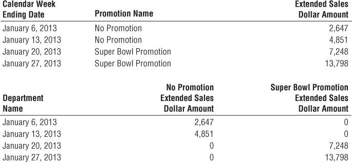
If the query tool summed the sales dollar amount grouped by week ending date and promotion, the SQL query results would look similar to those below inFigure 3.13. You can plainly see the relationship between the dimensional model and the associated query. High-quality dimension attributes are crucial because they are the source of query constraints and report labels. If you use a BI tool with more functionality, the results would likely appear as a cross-tabular “pivoted” report, which may be more appealing to business users than the columnar data resulting from an SQL statement.

Figure 3.13 Query results and cross-tabular report.

Retail Schema Extensibility

Let's turn our attention to extending the initial dimensional design. Several years after the rollout of the retail sales schema, the retailer implements a frequent shopper program. Rather than knowing an unidentified shopper purchased 26 items on a cash register receipt, you can now identify the specific shopper. Just imagine the business users' interest in analyzing shopping patterns by a multitude of geographic, demographic, behavioral, and other differentiating shopper characteristics.

The handling of this new frequent shopper information is relatively straightforward. You'd create a frequent shopper dimension table and add another foreign key in the fact table. Because you can't ask shoppers to bring in all their old cash register receipts to tag their historical sales transactions with their new frequent shopper number, you'd substitute a default shopper dimension surrogate key, corresponding to a Prior to Frequent Shopper Program dimension row, on the historical fact table rows. Likewise, not everyone who shops at the grocery store will have a frequent shopper card, so you'd also want to include a Frequent Shopper Not Identified row in the shopper dimension. As we discussed earlier with the promotion dimension, you can't have a null frequent shopper key in the fact table.

Our original schema gracefully extends to accommodate this new dimension largely because the POS transaction data was initially modeled at its most granular level. The addition of dimensions applicable at that granularity did not alter the existing dimension keys or facts; all existing BI applications continue to run without any changes. If the grain was originally declared as daily retail sales (transactions summarized by day, store, product, and promotion) rather than the transaction line detail, you would not have been able to incorporate the frequent shopper dimension. Premature summarization or aggregation inherently limits your ability to add supplemental dimensions because the additional dimensions often don't apply at the higher grain.

The predictable symmetry of dimensional models enable them to absorb some rather significant changes in source data and/or modeling assumptions without invalidating existing BI applications, including:

• New dimension attributes. If you discover new textual descriptors of a dimension, you can add these attributes as new columns. All existing applications will be oblivious to the new attributes and continue to function. If the new attributes are available only after a specific point in time, then Not Available or its equivalent should be populated in the old dimension rows. Be forewarned that this scenario is more complicated if the business users want to track historical changes to this newly identified attribute. If this is the case, pay close attention to the slowly changing dimension coverage in Chapter 5.
• New dimensions. As we just discussed, you can add a dimension to an existing fact table by adding a new foreign key column and populating it correctly with values of the primary key from the new dimension.
• New measured facts. If new measured facts become available, you can add them gracefully to the fact table. The simplest case is when the new facts are available in the same measurement event and at the same grain as the existing facts. In this case, the fact table is altered to add the new columns, and the values are populated into the table. If the new facts are only available from a point in time forward, null values need to be placed in the older fact rows.A more complex situation arises when new measured facts occur naturally at a different grain. If the new facts cannot be allocated or assigned to the original grain of the fact table, the new facts belong in their own fact table because it's a mistake to mix grains in the same fact table.

Factless Fact Tables

There is one important question that cannot be answered by the previous retail sales schema: What products were on promotion but did not sell? The sales fact table records only the SKUs actually sold. There are no fact table rows with zero facts for SKUs that didn't sell because doing so would enlarge the fact table enormously.

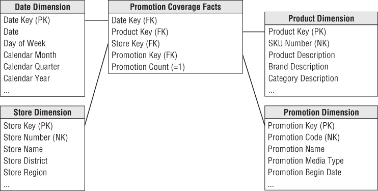
In the relational world, a promotion coverage or event fact table is needed to answer the question concerning what didn't happen. The promotion coverage fact table keys would be date, product, store, and promotion in this case study. This obviously looks similar to the sales fact table you just designed; however, the grain would be significantly different. In the case of the promotion coverage fact table, you'd load one row for each product on promotion in a store each day (or week, if retail promotions are a week in duration) regardless of whether the product sold. This fact table enables you to see the relationship between the keys as defined by a promotion, independent of other events, such as actual product sales. We refer to it as a factless fact table because it has no measurement metrics; it merely captures the relationship between the involved keys, as illustrated in Figure 3.14. To facilitate counting, you can include a dummy fact, such as promotion count in this example, which always contains the constant value of 1; this is a cosmetic enhancement that enables the BI application to avoid counting one of the foreign keys.

Figure 3.14 Promotion coverage factless fact table.

To determine what products were on promotion but didn't sell requires a two-step process. First, you'd query the promotion factless fact table to determine the universe of products that were on promotion on a given day. You'd then determine what products sold from the POS sales fact table. The answer to our original question is the set difference between these two lists of products. If you work with data in an OLAP cube, it is often easier to answer the “what didn't happen” question because the cube typically contains explicit cells for nonbehavior.

Dimension and Fact Table Keys

Now that the schemas have been designed, we'll focus on the dimension and fact tables' primary keys, along with other row identifiers.

Dimension Table Surrogate Keys

The unique primary key of a dimension table should be a surrogate key rather than relying on the operational system identifier, known as the natural key. Surrogate keys go by many other aliases: meaningless keys, integer keys, non-natural keys, artificial keys, and synthetic keys. Surrogate keys are simply integers that are assigned sequentially as needed to populate a dimension. The first product row is assigned a product surrogate key with the value of 1; the next product row is assigned product key 2; and so forth. The actual surrogate key value has no business significance. The surrogate keys merely serve to join the dimension tables to the fact table. Throughout this book, column names with a Key suffix, identified as a primary key (PK) or foreign key (FK), imply a surrogate.

Modelers sometimes are reluctant to relinquish the natural keys because they want to navigate the fact table based on the operational code while avoiding a join to the dimension table. They also don't want to lose the embedded intelligence that's often part of a natural multipart key. However, you should avoid relying on intelligent dimension keys because any assumptions you make eventually may be invalidated. Likewise, queries and data access applications should not have any built-in dependency on the keys because the logic also would be vulnerable to invalidation. Even if the natural keys appear to be stable and devoid of meaning, don't be tempted to use them as the dimension table's primary key.

Initially, it may be faster to implement a dimensional model using operational natural keys, but surrogate keys pay off in the long run. We sometimes think of them as being similar to a flu shot for the data warehouse—like an immunization, there's a small amount of pain to initiate and administer surrogate keys, but the long run benefits are substantial, especially considering the reduced risk of substantial rework. Here are several advantages:

• Buffer the data warehouse from operational changes. Surrogate keys enable the warehouse team to maintain control of the DW/BI environment rather than being whipsawed by operational rules for generating, updating, deleting, recycling, and reusing production codes. In many organizations, historical operational codes, such as inactive account numbers or obsolete product codes, get reassigned after a period of dormancy. If account numbers get recycled following 12 months of inactivity, the operational systems don't miss a beat because their business rules prohibit data from hanging around for that long. But the DW/BI system may retain data for years. Surrogate keys provide the warehouse with a mechanism to differentiate these two separate instances of the same operational account number. If you rely solely on operational codes, you might also be vulnerable to key overlaps in the case of an acquisition or consolidation of data.
• Integrate multiple source systems. Surrogate keys enable the data warehouse team to integrate data from multiple operational source systems, even if they lack consistent source keys by using a back room cross-reference mapping table to link the multiple natural keys to a common surrogate.
• Improve performance. The surrogate key is as small an integer as possible while ensuring it will comfortably accommodate the future anticipated cardinality (number of rows in the dimension). Often the operational code is a bulky alphanumeric character string or even a group of fields. The smaller surrogate key translates into smaller fact tables, smaller fact table indexes, and more fact table rows per block input–output operation. Typically, a 4-byte integer is sufficient to handle most dimensions. A 4-byte integer is a single integer, not four decimal digits. It has 32 bits and therefore can handle approximately 2 billion positive values (2³²) or 4 billion total positive and negative values (−2³² to +2³²). This is more than enough for just about any dimension. Remember, if you have a large fact table with 1 billion rows of data, every byte in each fact table row translates into another gigabyte of storage.
• Handle null or unknown conditions. As mentioned earlier, special surrogate key values are used to record dimension conditions that may not have an operational code, such as the No Promotion condition or the anonymous customer. You can assign a surrogate key to identify these despite the lack of operational coding. Similarly, fact tables sometimes have dates that are yet to be determined. There is no SQL date type value for Date to Be Determined or Date Not Applicable.
• Support dimension attribute change tracking. One of the primary techniques for handling changes to dimension attributes relies on surrogate keys to handle the multiple profiles for a single natural key. This is actually one of the most important reasons to use surrogate keys, which we'll describe in Chapter 5. A pseudo surrogate key created by simply gluing together the natural key with a time stamp is perilous. You need to avoid multiple joins between the dimension and fact tables, sometimes referred to as double-barreled joins, due to their adverse impact on performance and ease of use.

Of course, some effort is required to assign and administer surrogate keys, but it's not nearly as intimidating as many people imagine. You need to establish and maintain a cross-reference table in the ETL system that will be used to substitute the appropriate surrogate key on each fact and dimension table row. We lay out a process for administering surrogate keys in Chapter 19: ETL Subsystems and Techniques.

Dimension Natural and Durable Supernatural Keys

Like surrogate keys, the natural keys assigned and used by operational source systems go by other names, such as business keys, production keys, and operational keys. They are identified with the NK notation in the book's figures. The natural key is often modeled as an attribute in the dimension table. If the natural key comes from multiple sources, you might use a character data type that prepends a source code, such as SAP|43251 or CRM|6539152. If the same entity is represented in both operational source systems, then you'd likely have two natural key attributes in the dimension corresponding to both sources. Operational natural keys are often composed of meaningful constituent parts, such as the product's line of business or country of origin; these components should be split apart and made available as separate attributes.

In a dimension table with attribute change tracking, it's important to have an identifier that uniquely and reliably identifies the dimension entity across its attribute changes. Although the operational natural key may seem to fit this bill, sometimes the natural key changes due to unexpected business rules (like an organizational merger) or to handle either duplicate entries or data integration from multiple sources. If the dimension's natural keys are not absolutely protected and preserved over time, the ETL system needs to assign permanent durable identifiers, also known as supernatural keys. A persistent durable supernatural key is controlled by the DW/BI system and remains immutable for the life of the system. Like the dimension surrogate key, it's a simple integer sequentially assigned. And like the natural keys discussed earlier, the durable supernatural key is handled as a dimension attribute; it's not a replacement for the dimension table's surrogate primary key. Chapter 19 also discusses the ETL system's responsibility for these durable identifiers.

Degenerate Dimension Surrogate Keys

Although surrogate keys aren't typically assigned to degenerate dimensions, each situation needs to be evaluated to determine if one is required. A surrogate key is necessary if the transaction control numbers are not unique across locations or get reused. For example, the retailer's POS system may not assign unique transaction numbers across stores. The system may wrap back to zero and reuse previous control numbers when its maximum has been reached. Also, the transaction control number may be a bulky 24-byte alphanumeric column. Finally, depending on the capabilities of the BI tool, you may need to assign a surrogate key (and create an associated dimension table) to drill across on the transaction number. Obviously, control number dimensions modeled in this way with corresponding dimension tables are no longer degenerate.

Date Dimension Smart Keys

As we've noted, the date dimension has unique characteristics and requirements. Calendar dates are fixed and predetermined; you never need to worry about deleting dates or handling new, unexpected dates on the calendar. Because of its predictability, you can use a more intelligent key for the date dimension.

If a sequential integer serves as the primary key of the date dimension, it should be chronologically assigned. In other words, January 1 of the first year would be assigned surrogate key value 1, January 2 would be assigned surrogate key 2, February 1 would be assigned surrogate key 32, and so on.

More commonly, the primary key of the date dimension is a meaningful integer formatted as yyyymmdd. The yyyymmdd key is not intended to provide business users and their BI applications with an intelligent key so they can bypass the date dimension and directly query the fact table. Filtering on the fact table's yyyymmdd key would have a detrimental impact on usability and performance. Filtering and grouping on calendar attributes should occur in a dimension table, not in the BI application's code.

However, the yyyymmdd key is useful for partitioning fact tables. Partitioning enables a table to be segmented into smaller tables under the covers. Partitioning a large fact table on the basis of date is effective because it allows old data to be removed gracefully and new data to be loaded and indexed in the current partition without disturbing the rest of the fact table. It reduces the time required for loads, backups, archiving, and query response. Programmatically updating and maintaining partitions is straightforward if the date key is an ordered integer: year increments by 1 up to the number of years wanted, month increments by 1 up to 12, and so on. Using a smart yyyymmdd key provides the benefits of a surrogate, plus the advantages of easier partition management.

Although the yyyymmdd integer is the most common approach for date dimension keys, some relational database optimizers prefer a true date type column for partitioning. In these cases, the optimizer knows there are 31 values between March 1 and April 1, as opposed to the apparent 100 values between 20130301 and 20130401. Likewise, it understands there are 31 values between December 1 and January 1, as opposed to the 8,900 integer values between 20121201 and 20130101. This intelligence can impact the query strategy chosen by the optimizer and further reduce query times. If the optimizer incorporates date type intelligence, it should be considered for the date key. If the only rationale for a date type key is simplified administration for the DBA, then you can feel less compelled.

With more intelligent date keys, whether chronologically assigned or a more meaningful yyyymmdd integer or date type column, you need to reserve a special date key value for the situation in which the date is unknown when the fact row is initially loaded.

Fact Table Surrogate Keys

Although we're adamant about using surrogate keys for dimension tables, we're less demanding about a surrogate key for fact tables. Fact table surrogate keys typically only make sense for back room ETL processing. As we mentioned, the primary key of a fact table typically consists of a subset of the table's foreign keys and/or degenerate dimension. However, single column surrogate keys for fact tables have some interesting back room benefits.

Like its dimensional counterpart, a fact table surrogate key is a simple integer, devoid of any business content, that is assigned in sequence as fact table rows are generated. Although the fact table surrogate key is unlikely to deliver query performance advantages, it does have the following benefits:

• Immediate unique identification. A single fact table row is immediately identified by the key. During ETL processing, a specific row can be identified without navigating multiple dimensions.
• Backing out or resuming a bulk load. If a large number of rows are being loaded with sequentially assigned surrogate keys, and the process halts before completion, the DBA can determine exactly where the process stopped by finding the maximum key in the table. The DBA could back out the complete load by specifying the range of keys just loaded or perhaps could resume the load from exactly the correct point.
• Replacing updates with inserts plus deletes. The fact table surrogate key becomes the true physical key of the fact table. No longer is the key of the fact table determined by a set of dimensional foreign keys, at least as far as the RDBMS is concerned. Thus it becomes possible to replace a fact table update operation with an insert followed by a delete. The first step is to place the new row into the database with all the same business foreign keys as the row it is to replace. This is now possible because the key enforcement depends only on the surrogate key, and the replacement row has a new surrogate key. Then the second step deletes the original row, thereby accomplishing the update. For a large set of updates, this sequence is more efficient than a set of true update operations. The insertions can be processed with the ability to back out or resume the insertions as described in the previous bullet. These insertions do not need to be protected with full transaction machinery. Then the final deletion step can be performed safely because the insertions have run to completion.
• Using the fact table surrogate key as a parent in a parent/child schema. In those cases in which one fact table contains rows that are parents of those in a lower grain fact table, the fact table surrogate key in the parent table is also exposed in the child table. The argument of using the fact table surrogate key in this case rather than a natural parent key is similar to the argument for using surrogate keys in dimension tables. Natural keys are messy and unpredictable, whereas surrogate keys are clean integers and are assigned by the ETL system, not the source system. Of course, in addition to including the parent fact table's surrogate key, the lower grained fact table should also include the parent's dimension foreign keys so the child facts can be sliced and diced without traversing the parent fact table's surrogate key. And as we'll discuss in Chapter 4: Inventory, you should never join fact tables directly to other fact tables.

Resisting Normalization Urges

In this section, let's directly confront several of the natural urges that tempt modelers coming from a more normalized background. We've been consciously breaking some traditional modeling rules because we're focused on delivering value through ease of use and performance, not on transaction processing efficiencies.

Snowflake Schemas with Normalized Dimensions

The flattened, denormalized dimension tables with repeating textual values make data modelers from the operational world uncomfortable. Let's revisit the case study product dimension table. The 300,000 products roll up into 50 distinct departments. Rather than redundantly storing the 20-byte department description in the product dimension table, modelers with a normalized upbringing want to store a 2-byte department code and then create a new department dimension for the department decodes. In fact, they would feel more comfortable if all the descriptors in the original design were normalized into separate dimension tables. They argue this design saves space because the 300,000-row dimension table only contains codes, not lengthy descriptors.

In addition, some modelers contend that more normalized dimension tables are easier to maintain. If a department description changes, they'd need to update only the one occurrence in the department dimension rather than the 6,000 repetitions in the original product dimension. Maintenance often is addressed by normalization disciplines, but all this happens back in the ETL system long before the data is loaded into a presentation area's dimensional schema.

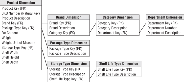
Dimension table normalization is referred to as snowflaking. Redundant attributes are removed from the flat, denormalized dimension table and placed in separate normalized dimension tables. Figure 3.15 illustrates the partial snowflaking of the product dimension into third normal form. The contrast between Figure 3.15 and Figure 3.8 is startling. The plethora of snowflaked tables (even in our simplistic example) is overwhelming. Imagine the impact on Figure 3.12 if all the schema's hierarchies were normalized.

Figure 3.15 Snowflaked product dimension.

Snowflaking is a legal extension of the dimensional model, however, we encourage you to resist the urge to snowflake given the two primary design drivers: ease of use and performance.

• The multitude of snowflaked tables makes for a much more complex presentation. Business users inevitably will struggle with the complexity; simplicity is one of the primary objectives of a dimensional model.
• Most database optimizers also struggle with the snowflaked schema's complexity. Numerous tables and joins usually translate into slower query performance. The complexities of the resulting join specifications increase the chances that the optimizer will get sidetracked and choose a poor strategy.
• The minor disk space savings associated with snowflaked dimension tables are insignificant. If you replace the 20-byte department description in the 300,000 row product dimension table with a 2-byte code, you'd save a whopping 5.4 MB (300,000 x 18 bytes); meanwhile, you may have a 10 GB fact table! Dimension tables are almost always geometrically smaller than fact tables. Efforts to normalize dimension tables to save disk space are usually a waste of time.
• Snowflaking negatively impacts the users' ability to browse within a dimension. Browsing often involves constraining one or more dimension attributes and looking at the distinct values of another attribute in the presence of these constraints. Browsing allows users to understand the relationship between dimension attribute values.
• Obviously, a snowflaked product dimension table responds well if you just want a list of the category descriptions. However, if you want to see all the brands within a category, you need to traverse the brand and category dimensions. If you want to also list the package types for each brand in a category, you'd be traversing even more tables. The SQL needed to perform these seemingly simple queries is complex, and you haven't touched the other dimensions or fact table.
• Finally, snowflaking defeats the use of bitmap indexes. Bitmap indexes are useful when indexing low-cardinality columns, such as the category and department attributes in the product dimension table. They greatly speed the performance of a query or constraint on the single column in question. Snowflaking inevitably would interfere with your ability to leverage this performance tuning technique.

Some database vendors argue their platform has the horsepower to query a fully normalized dimensional model without performance penalties. If you can achieve satisfactory performance without physically denormalizing the dimension tables, that's fine. However, you'll still want to implement a logical dimensional model with denormalized dimensions to present an easily understood schema to the business users and their BI applications.

In the past, some BI tools indicated a preference for snowflake schemas; snowflaking to address the idiosyncratic requirements of a BI tool is acceptable. Likewise, if all the data is delivered to business users via an OLAP cube (where the snowflaked dimensions are used to populate the cube but are never visible to the users), then snowflaking is acceptable. However, in these situations, you need to consider the impact on users of alternative BI tools and the flexibility to migrate to alternatives in the future.

Outriggers

Although we generally do not recommend snowflaking, there are situations in which it is permissible to build an outrigger dimension that attaches to a dimension within the fact table's immediate halo, as illustrated in Figure 3.16. In this example, the “once removed” outrigger is a date dimension snowflaked off a primary dimension. The outrigger date attributes are descriptively and uniquely labeled to distinguish them from the other dates associated with the business process. It only makes sense to outrigger a primary dimension table's date attribute if the business wants to filter and group this date by nonstandard calendar attributes, such as the fiscal period, business day indicator, or holiday period. Otherwise, you could just treat the date attribute as a standard date type column in the product dimension. If a date outrigger is used, be careful that the outrigger dates fall within the range stored in the standard date dimension table.

Figure 3.16 Example of a permissible outrigger.

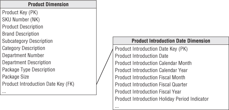
You'll encounter more outrigger examples later in the book, such as the handling of customers' county-level demographic attributes in Chapter 8: Customer Relationship Management.

Although outriggers may save space and ensure the same attributes are referenced consistently, there are downsides. Outriggers introduce more joins, which can negatively impact performance. More important, outriggers can negatively impact the legibility for business users and hamper their ability to browse among attributes within a single dimension.

Centipede Fact Tables with Too Many Dimensions

The fact table in a dimensional schema is naturally highly normalized and compact. There is no way to further normalize the extremely complex many-to-many relationships among the keys in the fact table because the dimensions are not correlated with each other. Every store is open every day. Sooner or later, almost every product is sold on promotion in most or all of our stores.

Interestingly, while uncomfortable with denormalized dimension tables, some modelers are tempted to denormalize the fact table. They have an uncontrollable urge to normalize dimension hierarchies but know snowflaking is highly discouraged, so the normalized tables end up joined to the fact table instead. Rather than having a single product foreign key on the fact table, they include foreign keys for the frequently analyzed elements on the product hierarchy, such as brand, category, and department. Likewise, the date key suddenly turns into a series of keys joining to separate week, month, quarter, and year dimension tables. Before you know it, your compact fact table has turned into an unruly monster that joins to literally dozens of dimension tables. We affectionately refer to these designs as centipede fact tables because they appear to have nearly 100 legs, as shown in Figure 3.17.

Figure 3.17 Centipede fact table with too many normalized dimensions.

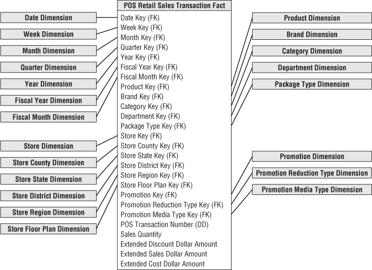
Even with its tight format, the fact table is the behemoth in a dimensional model. Designing a fact table with too many dimensions leads to significantly increased fact table disk space requirements. Although denormalized dimension tables consume extra space, fact table space consumption is a concern because it is your largest table by orders of magnitude. There is no way to index the enormous multipart key effectively in the centipede example. The numerous joins are an issue for both usability and query performance.

Most business processes can be represented with less than 20 dimensions in the fact table. If a design has 25 or more dimensions, you should look for ways to combine correlated dimensions into a single dimension. Perfectly correlated attributes, such as the levels of a hierarchy, as well as attributes with a reasonable statistical correlation, should be part of the same dimension. It's a good decision to combine dimensions when the resulting new single dimension is noticeably smaller than the Cartesian product of the separate dimensions.

Developments with columnar databases may reduce the query and storage penalties associated with wide centipede fact table designs. Rather than storing each table row, a columnar database stores each table column as a contiguous object that is heavily indexed for access. Even though the underlying physical storage is columnar, at the query level, the table appears to be made up of familiar rows. But when queried, only the named columns are actually retrieved from the disk, rather than the entire row in a more conventional row-oriented relational database. Columnar databases are much more tolerant of the centipede fact tables just described; however, the ability to browse across hierarchically related dimension attributes may be compromised.

Summary

This chapter was your first exposure to designing a dimensional model. Regardless of the industry, we strongly encourage the four-step process for tackling dimensional model designs. Remember it is especially important to clearly state the grain associated with a dimensional schema. Loading the fact table with atomic data provides the greatest flexibility because the data can be summarized “every which way.” As soon as the fact table is restricted to more aggregated information, you run into walls when the summarization assumptions prove to be invalid. Also it is vitally important to populate your dimension tables with verbose, robust descriptive attributes for analytic filtering and labeling.

In the next chapter we'll remain within the retail industry to discuss techniques for tackling a second business process within the organization, ensuring your earlier efforts are leveraged while avoiding stovepipes.