
1. Introduction to Data Wrangling with Python
Activity 1.01: Handling Lists
Solution:
These are the steps to complete this activity:
- Import the random library:
import random
- Use the randint method from the random library to create 100 random numbers:
random_number_list = [random.randint(0, 100)
for x in range(0, 100)]
- Print random_number_list:
random_number_list
The sample output is as follows:
Figure 1.20: Section of output for random_number_list
Note
The output is susceptible to change since we are generating random numbers.
- Create a list_with_divisible_by_3 list from random_number_list, which will contain only numbers that are divisible by 3:
list_with_divisible_by_3 = [a for a in
random_number_list if a % 3 == 0]
list_with_divisible_by_3
The sample output is as follows:
Figure 1.21: Section of the output for random_number_list divisible by 3
- Use the len function to measure the length of the first list and the second list, and store them in two different variables, length_of_random_list and length_of_3_divisible_list. Calculate the difference in length in a variable called difference:
length_of_random_list = len(random_number_list)
length_of_3_divisible_list = len(list_with_divisible_by_3)
difference = length_of_random_list - length_of_3_divisible_list
difference
The sample output is as follows:
71
- Combine the tasks we have performed so far and add a for loop to it. Run the loop 10 times and add the values of the difference variables to a list:
NUMBER_OF_EXPERIMENTS = 10
difference_list = []
for i in range(0, NUMBER_OF_EXPERIMENTS):
random_number_list = [random.randint(0, 100)
for x in range(0, 100)]
list_with_divisible_by_3 = [a for a in random_number_list
if a % 3 == 0]
length_of_random_list = len(random_number_list)
length_of_3_divisible_list = len(list_with_divisible_by_3)
difference = length_of_random_list
- length_of_3_divisible_list
difference_list.append(difference)
difference_list
The sample output is as follows:
[64, 61, 67, 60, 73, 66, 66, 75, 70, 61]
- Then, calculate the arithmetic mean (common average) for the differences in the lengths that you have:
avg_diff = sum(difference_list) / float(len(difference_list))
avg_diff
The sample output is as follows:
66.3
Note
The output is susceptible to change since we have used random numbers.
To access the source code for this specific section, please refer to https://packt.live/30VMjt3.
You can also run this example online at https://packt.live/3eh0JIb.
With this, we have successfully completed our first activity. Let's move on to the next section, where we will discuss another type of data structure – sets.
Activity 1.02: Analyzing a Multiline String and Generating the Unique Word Count
Solution:
These are the steps to complete this activity:
- Open a new Jupyter Notebook, create a string called multiline_text, and copy the text present in the first chapter of Pride and Prejudice.
Note
Part of the first chapter of Pride and Prejudice by Jane Austen has been made available on this book's GitHub repository at https://packt.live/2N6ZGP6.
Use Ctrl + A to select the entire text and then Ctrl + C to copy it and use Ctrl + V to paste the text you just copied into it:
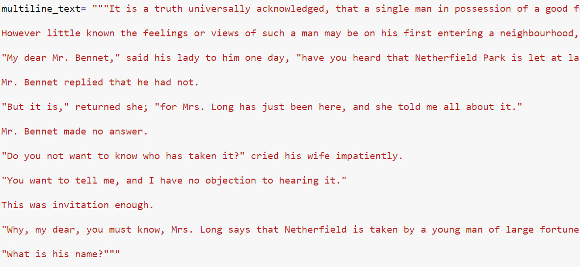
Figure 1.22: Initializing the mutliline_text string
- Find the type of the string using the type function:
type(multiline_text)
The output is as follows:
str
- Now, find the length of the string using the len function:
len(multiline_text)
The output is as follows:
1228
- Use string methods to get rid of all the new lines (
or
) and symbols. Remove all new lines by replacing them with the following:
multiline_text = multiline_text.replace(' ', "")
- Then, we will print and check the output:
multiline_text
The output is as follows:
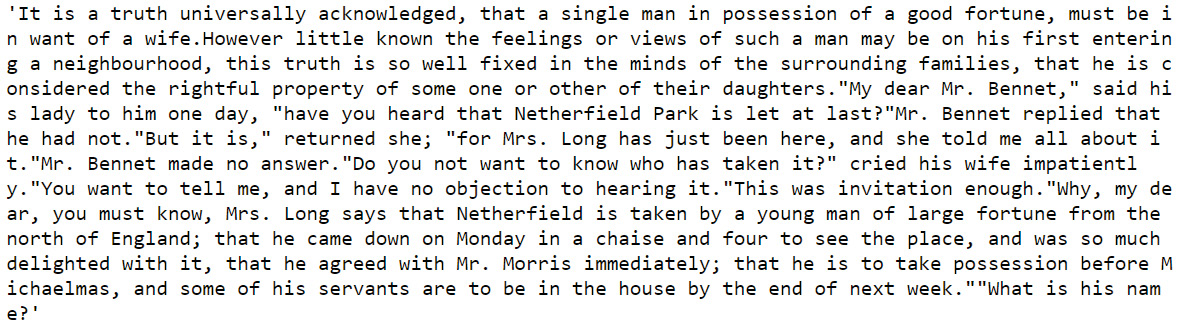
Figure 1.23: The multiline_text string after removing the new lines
- Remove the special characters and punctuation:
# remove special chars, punctuation etc.
cleaned_multiline_text = ""
for char in multiline_text:
if char == " ":
cleaned_multiline_text += char
elif char.isalnum(): # using the isalnum() method of strings.
cleaned_multiline_text += char
else:
cleaned_multiline_text += " "
- Check the content of cleaned_multiline_text:
cleaned_multiline_text
The output is as follows:

Figure 1.24: The cleaned_multiline_text string
- Generate a list of all the words from the cleaned string using the following command:
list_of_words = cleaned_multiline_text.split()
list_of_words
The section of the output is shown below:
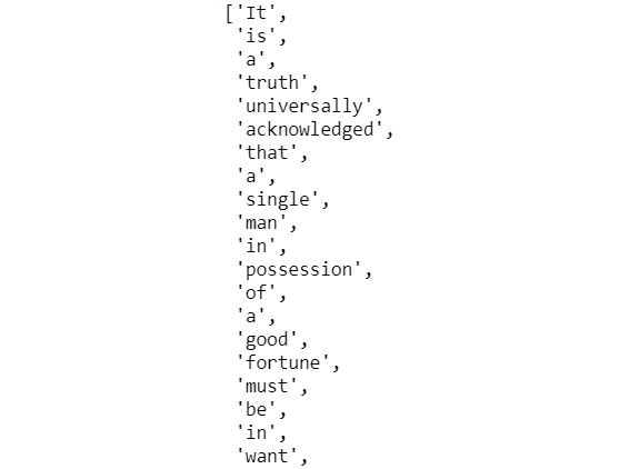
Figure 1.25: The section of output displaying the list_of_words
- Find the number of words:
len(list_of_words)
The output is 236.
- Create a list from the list you just created, which includes only unique words:
unique_words_as_dict = dict.fromkeys(list_of_words)
len(list(unique_words_as_dict.keys()))
The output is 135.
- Count the number of times each of the unique words appeared in the cleaned text:
for word in list_of_words:
if unique_words_as_dict[word] is None:
unique_words_as_dict[word] = 1
else:
unique_words_as_dict[word] += 1
unique_words_as_dict
The section of the output is shown below:
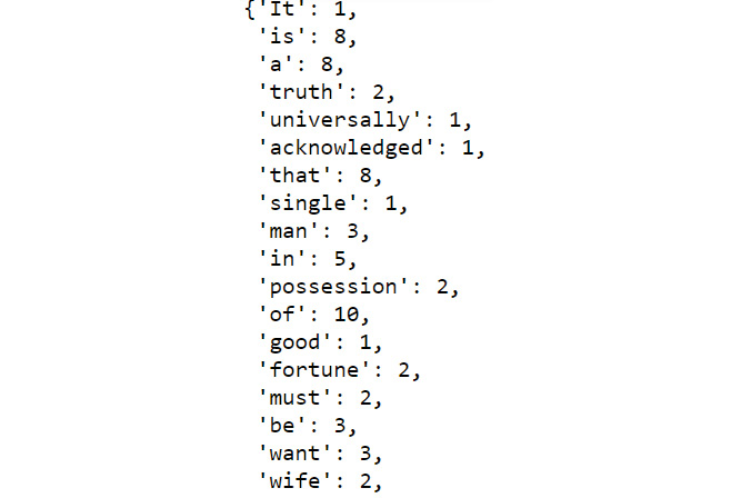
Figure 1.26: Section of output showing unique_words_as_dict
You just created, step by step, a unique word counter using all the neat tricks that you've learned about in this chapter.
- Find the top 25 words from unique_words_as_dict:
top_words = sorted(unique_words_as_dict.items(),
key=lambda key_val_tuple: key_val_tuple[1],
reverse=True)
top_words[:25]
The output (partially shown) is as follows:
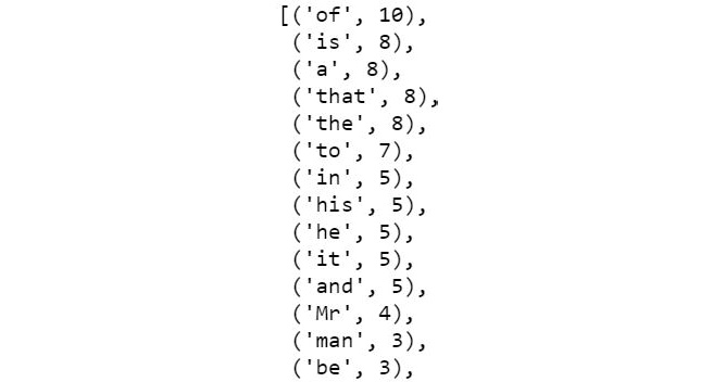
Figure 1.27: Top 25 unique words from multiline_text
Note
To access the source code for this specific section, please refer to https://packt.live/2ASNIWL.
You can also run this example online at https://packt.live/3dcIKkz.
2. Advanced Operations on Built-In Data Structures
Activity 2.01: Permutation, Iterator, Lambda, and List
Solution:
These are the detailed steps to solve this activity:
- Look up the definition of permutations and dropwhile from itertools. There is a way to look up the definition of a function inside Jupyter itself. Just type the function name, followed by ?, and press Shift + Enter:
from itertools import permutations, dropwhile
permutations?
dropwhile?
You will see a long list of definitions after each ?. We will skip it here.
- Write an expression to generate all the possible three-digit numbers using 1, 2, and 3:
permutations(range(3))
The output (which will vary in your case) is as follows:
<itertools.permutations at 0x7f6c6c077af0>
- Loop over the iterator expression you generated before. Use the print method to print each element returned by the iterator. Use assert and isinstance to make sure that the elements are tuples:
for number_tuple in permutations(range(3)):
print(number_tuple)
assert isinstance(number_tuple, tuple)
The output is as follows:
(0, 1, 2)
(0, 2, 1)
(1, 0, 2)
(1, 2, 0)
(2, 0, 1)
(2, 1, 0)
- Write the loop again. But this time, use dropwhile with a lambda expression to drop any leading zeros from the tuples. As an example, (0, 1, 2) will become [0, 2]. Also, cast the output of dropwhile to a list.
An extra task can be to check the actual type that dropwhile returns without casting:
for number_tuple in permutations(range(3)):
print(list(dropwhile(lambda x: x <= 0, number_tuple)))
The output is as follows:
[1, 2]
[2, 1]
[1, 0, 2]
[1, 2, 0]
[2, 0, 1]
[2, 1, 0]
- Write all the logic you wrote before, but this time write a separate function where you will be passing the list generated from dropwhile; the function will return the whole number contained in the list. As an example, if you pass [1, 2] to the function, it will return 12. Make sure that the return type is indeed a number and not a string. Although this task can be achieved using other tricks, we require you to treat the incoming list as a stack in the function and generate the number there:
import math
def convert_to_number(number_stack):
final_number = 0
for i in range(0, len(number_stack)):
final_number += (number_stack.pop()
* (math.pow(10, i)))
return final_number
for number_tuple in permutations(range(3)):
number_stack = list(dropwhile(lambda x: x <= 0, number_tuple))
print(convert_to_number(number_stack))
The output is as follows:
12.0
21.0
102.0
120.0
201.0
210.0
Note
To access the source code for this specific section, please refer to https://packt.live/37Gk9DT.
You can also run this example online at https://packt.live/3hEWt7f.
Activity 2.02: Designing Your Own CSV Parser
Solution:
These are the detailed steps to solve this activity:
- Import zip_longest from itertools:
from itertools import zip_longest
- Define the return_dict_from_csv_line function so that it contains header, line, and fillvalue as None, and add it to a dictionary:
def return_dict_from_csv_line(header, line):
# Zip them
zipped_line = zip_longest(header, line, fillvalue=None)
# Use dict comprehension to generate the final dict
ret_dict = {kv[0]: kv[1] for kv in zipped_line}
return ret_dict
- Open the accompanying sales_record.csv file using r mode inside a with block. First, check that it is opened, read the first line, and use string methods to generate a list of all the column names as follows:
with open("../datasets/sales_record.csv", "r") as fd:
Note
Don't forget to change the path (highlighted) based on where you have stored the csv file.
- When you read each line, pass that line to a function along with the list of the headers. The work of the function is to construct a dictionary out of these two and fill up the key:values variables. Keep in mind that a missing value should result in None:
first_line = fd.readline()
header = first_line.replace(" ", "").split(",")
for i, line in enumerate(fd):
line = line.replace(" ", "").split(",")
d = return_dict_from_csv_line(header, line)
print(d)
if i > 10:
break
The output (partially shown) is as follows:
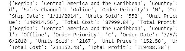
Figure 2.15: Section of output
Note
To access the source code for this specific section, please refer to https://packt.live/37FlVVK.
You can also run this example online at https://packt.live/2YepGyb.
3. Introduction to NumPy, Pandas, and Matplotlib
Activity 3.01: Generating Statistics from a CSV File
Solution:
These are the steps to complete this activity:
- Load the necessary libraries:
import numpy as np
import pandas as pd
import matplotlib.pyplot as plt
- Read in the Boston Housing dataset (given as a .csv file) from the local directory:
df=pd.read_csv("../datasets/Boston_housing.csv")
Note
Don't forget to change the path of the dataset (highlighted) based on where it is saved on your system.
- Check the first 10 records:
df.head(10)
The output is as follows:
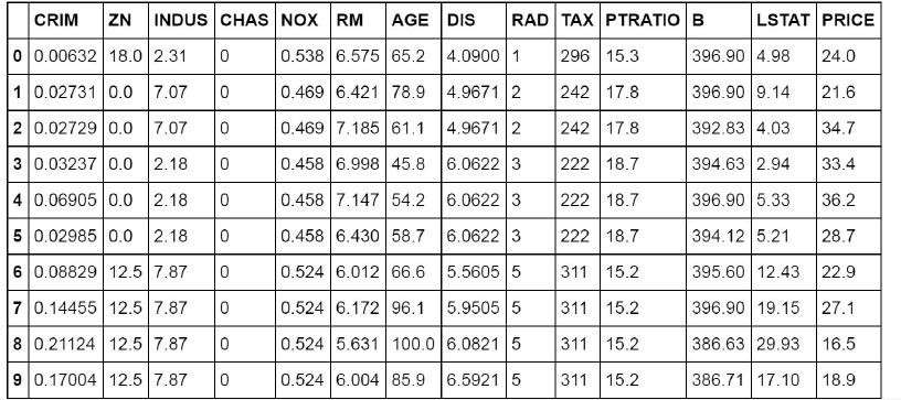
Figure 3.30: Output displaying the first 10 records
- Find the total number of records:
df.shape
The output is as follows:
(506, 14)
- Create a smaller DataFrame with columns that do not include CHAS, NOX, B, and LSTAT:
df1=df[['CRIM','ZN','INDUS',
'RM','AGE','DIS','RAD',
'TAX','PTRATIO','PRICE']]
- Check the last 7 records of the new DataFrame you just created:
df1.tail(7)
The output is as follows:
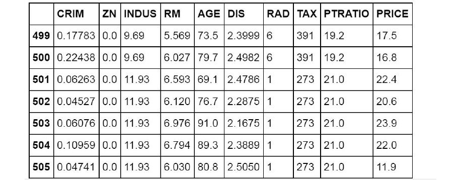
Figure 3.31: Last seven records of the DataFrame
- Plot histograms of all the variables (columns) in the new DataFrame by using a for loop:
for c in df1.columns:
plt.title("Plot of "+c,fontsize=15)
plt.hist(df1[c],bins=20)
plt.show()
The output is as follows:
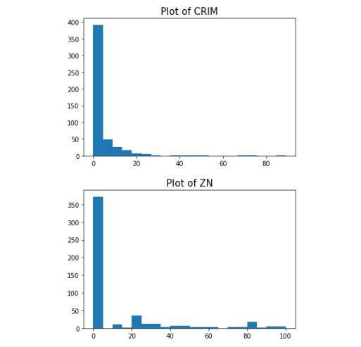
Figure 3.32: Partial plot of all variables using a for loop
Note
To take a look at all the plots, head over to the following link: https://packt.live/2AGb95F.
Crime rate could be an indicator of house price (people don't want to live in high-crime areas). In some cases, having multiple charts together can allow for the easy analysis of a variety of variables. In the preceding group of charts, we can see several unique spikes in the data: INDIUS, TAX, and RAD. With further exploratory analysis, we can find out more. We might want to plot one variable against another after looking at the preceding group of charts.
- Create a scatter plot of crime rate versus price:
plt.scatter(df1['CRIM'], df1['PRICE'])
plt.show()
The output is as follows:
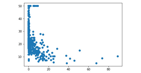
Figure 3.33: Scatter plot of crime rate versus price
We can understand this relationship better if we plot log10(crime) versus price.
- Create a plot of log10(crime) versus price:
plt.scatter(np.log10(df1['CRIM']),df1['PRICE'], c='red')
plt.title("Crime rate (Log) vs. Price plot", fontsize=18)
plt.xlabel("Log of Crime rate",fontsize=15)
plt.ylabel("Price",fontsize=15)
plt.grid(True)
plt.show()
The output is as follows:
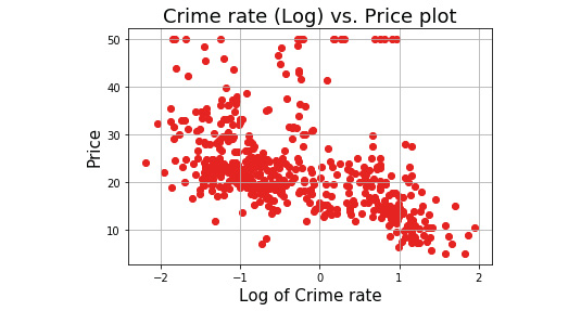
Figure 3.34: Scatter plot of crime rate (Log) versus price
- Calculate the mean rooms per dwelling:
df1['RM'].mean()
The output is as follows:
6.284634387351788
- Calculate the median age:
df1['AGE'].median()
The output is as follows:
77.5
- Calculate the average (mean) distances to five Boston employment centers:
df1['DIS'].mean()
The output is as follows:
3.795042687747034
- Calculate the price of the housing that's less than 20:
low_price=df1['PRICE']<20
print(low_price)
The output is as follows:
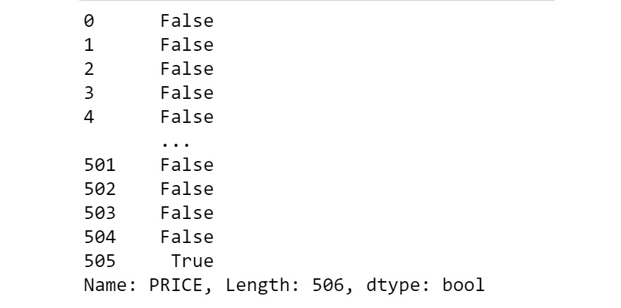
Figure 3.35: Output of low_price
This creates a Boolean array of True, False, True = 1, and False = 0. If you take an average of this NumPy array, you will know how many 1(True) values are there.
- Calculate the mean of this array:
# That many houses are priced below 20,000.
# So that is the answer.
low_price.mean()
The output is:
0.4150197628458498
- Calculate the percentage of houses with a low price (< $20,000):
# You can convert that into percentage
# Do this by multiplying with 100
pcnt=low_price.mean()*100
print(" Percentage of house with <20,000 price is: ", pcnt)
The output is as follows:
Percentage of house with <20,000 price is: 41.50197628458498
Note
To access the source code for this specific section, please refer to https://packt.live/2AGb95F.
You can also run this example online at https://packt.live/2YT3Hfg.
4. A Deep Dive into Data Wrangling with Python
Activity 4.01: Working with the Adult Income Dataset (UCI)
Solution:
These are the steps to complete this activity:
- Load the necessary libraries:
import numpy as np
import pandas as pd
import matplotlib.pyplot as plt
- Read in the Adult Income Dataset (given as a .csv file) from the local directory and check the first five records:
df = pd.read_csv("../datasets/adult_income_data.csv")
df.head()
Note
The highlighted path must be changed based on the location of the file on your system.
The output is as follows:
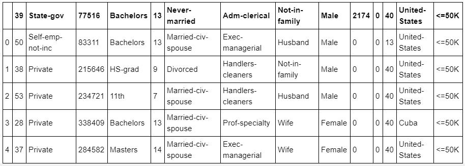
Figure 4.76: DataFrame displaying the first five records from the .csv file
- Create a script that will read a text file line by line and extract the first line, which is the header of the .csv file:
names = []
with open('../datasets/adult_income_names.txt','r') as f:
for line in f:
f.readline()
var=line.split(":")[0]
names.append(var)
names
Note
The highlighted path must be changed based on the location of the file on your system.
The output is as follows:
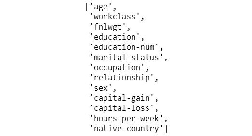
Figure 4.77: Names of the columns in the database
- Add a name of Income for the response variable (last column) to the dataset by using the append command:
names.append('Income')
- Read the new file again using the following command:
df = pd.read_csv("../datasets/adult_income_data.csv", names=names)
df.head()
Note
The highlighted path must be changed based on the location of the file on your system.
The output is as follows:
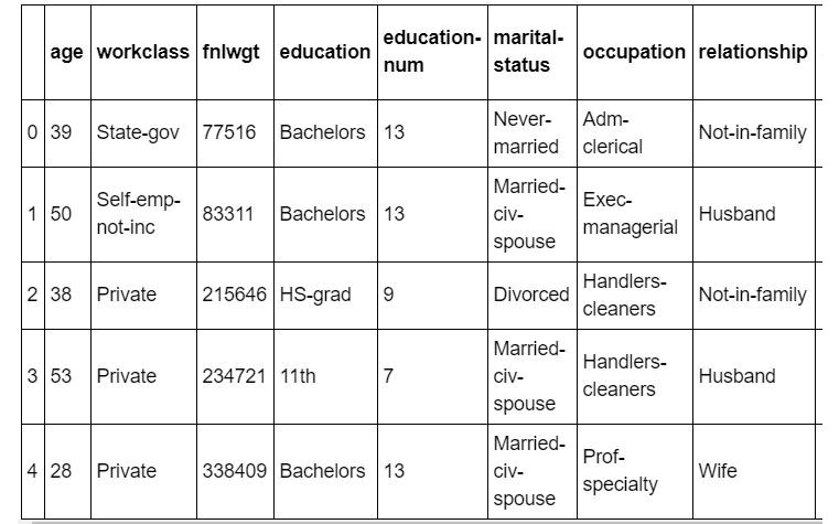
Figure 4.78: DataFrame with the income column added
- Use the describe command to get the statistical summary of the dataset:
df.describe()
The output is as follows:
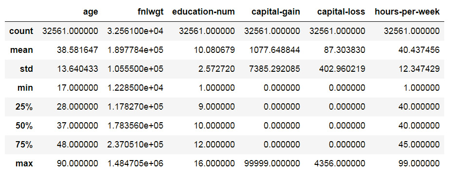
Figure 4.79: Statistical summary of the dataset
Note that only a small number of columns are included. Many variables in the dataset have multiple factors or classes.
- Make a list of all the variables in the classes by using the following command:
# Make a list of all variables with classes
vars_class = ['workclass','education','marital-status',
'occupation','relationship','sex','native-country']
- Create a loop to count and print them by using the following command:
for v in vars_class:
classes=df[v].unique()
num_classes = df[v].nunique()
print("There are {} classes in the "{}" column. "
"They are: {}".format(num_classes,v,classes))
print("-"*100)
The output (partially shown) is as follows:
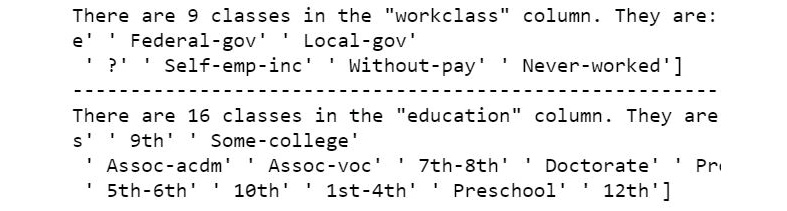
Figure 4.80: Output of different factors or classes
- Find the missing values by using the following command:
df.isnull().sum()
The output is as follows:
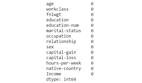
Figure 4.81: Finding the missing values
- Create a DataFrame with only age, education, and occupation by using subsetting:
df_subset = df[['age','education', 'occupation']]
df_subset.head()
The output is as follows:
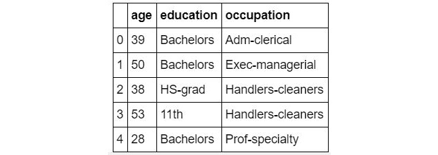
Figure 4.82: Subset of the DataFrame
- Plot a histogram of age with a bin size of 20:
df_subset['age'].hist(bins=20)
The output is as follows:
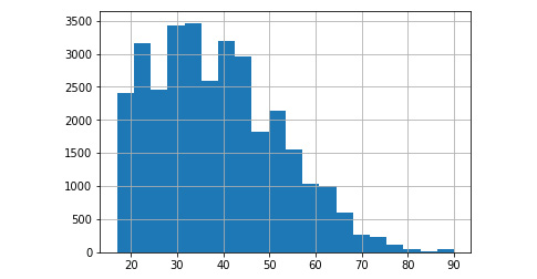
Figure 4.83: Histogram of age with a bin size of 20
- Plot box plots for age grouped by education (use a long figure size of 25x10 and make the x ticks font size 15):
df_subset.boxplot(column='age',by='education',figsize=(25,10))
plt.xticks(fontsize=15)
plt.xlabel("Education",fontsize=20)
plt.show()
The output is as follows:
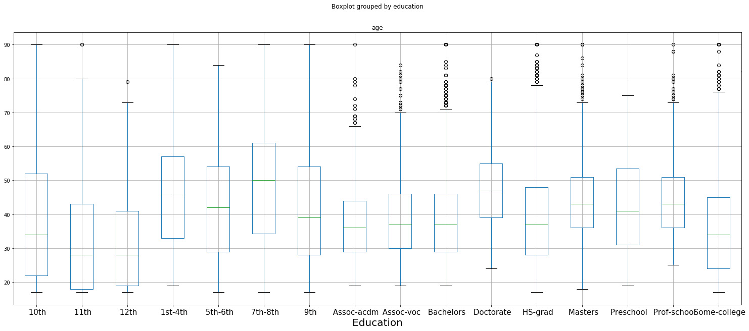
Figure 4.84: Box plot of age grouped by education
Before doing any further operations, we need to use the apply method we learned about in this chapter. It turns out that when reading the dataset from the CSV file, all the strings came with a whitespace character in front of them. So, we need to remove that whitespace from all the strings.
- Create a function to strip the whitespace characters:
def strip_whitespace(s):
return s.strip()
- Use the apply method to apply this function to all the columns with string values, create a new column, copy the values from this new column to the old column, and drop the new column. This is the preferred method so that you don't accidentally delete valuable data. Most of the time, you will need to create a new column with a desired operation and then copy it back to the old column if necessary. Ignore any warning messages that are printed:
# Education column
df_subset['education_stripped'] = df['education']
.apply(strip_whitespace)
df_subset['education'] = df_subset['education_stripped']
df_subset.drop(labels = ['education_stripped'],
axis=1,inplace=True)
# Occupation column
df_subset['occupation_stripped'] = df['occupation']
.apply(strip_whitespace)
df_subset['occupation'] = df_subset['occupation_stripped']
df_subset.drop(labels = ['occupation_stripped'],
axis=1,inplace=True)
This is the sample warning message, which you should ignore:
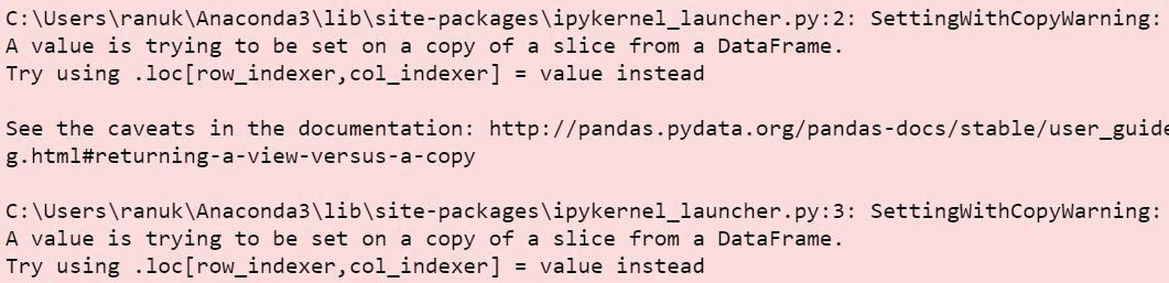
Figure 4.85: Warning message to be ignored
- Find the number of people who are aged between 30 and 50 (inclusive) by using the following command:
# Conditional clauses and join them by & (AND)
df_filtered=df_subset[(df_subset['age']>=30)
& (df_subset['age']<=50)]
- Check the contents of the new dataset:
df_filtered.head()
The output is as follows:
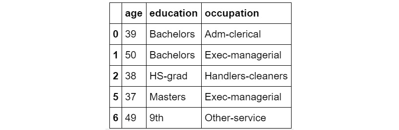
Figure 4.86: Contents of the new DataFrame
- Find the shape of the filtered DataFrame and specify the index of the tuple as 0 to return the first element:
answer_1=df_filtered.shape[0]
answer_1
The output is as follows:
16390
- Print the number of people aged between 30 and 50 using the following command:
print("There are {} people of age between 30 and 50 "
"in this dataset.".format(answer_1))
The output is as follows:
There are 16390 people of age between 30 and 50 in this dataset.
- Group by occupation and show the summary statistics of age. Find which profession has the oldest workers on average and which profession has its largest share of the workforce above the 75th percentile:
df_subset.groupby('occupation').describe()['age']
The output is as follows:
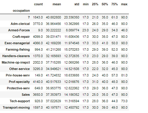
Figure 4.87: DataFrame with data grouped by age and education
The code returns 79 rows × 1 columns.
- Use subset and groupBy to find the outliers:
occupation_stats=df_subset.groupby('occupation').describe()['age']
- Plot the values on a bar chart:
plt.figure(figsize=(15,8))
plt.barh(y=occupation_stats.index,
width=occupation_stats['count'])
plt.yticks(fontsize=13)
plt.show()
The output is as follows:
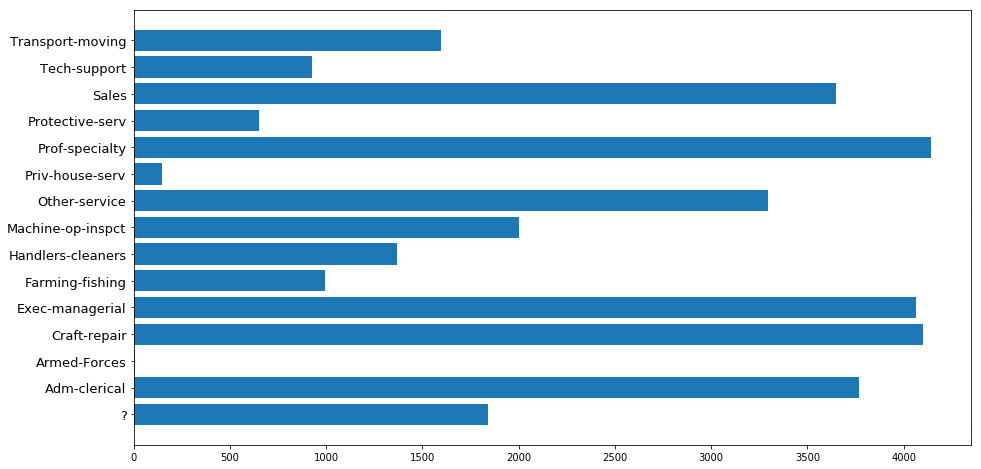
Figure 4.88: Bar chart displaying occupation statistics
Is there a particular occupation group that has very low representation? Perhaps we should remove those pieces of data because, with very low data, the group won't be useful in analysis. Just by looking at Figure 4.89, you should be able to see that the Armed-Forces group has only got a 9 count, that is, 9 data points. But how can we detect this? By plotting the count column in a bar chart. Note how the first argument to the barh function is the index of the DataFrame, which is the summary stats of the occupation groups. We can see that the Armed-Forces group has almost no data. This activity teaches you that, sometimes, the outlier is not just a value, but can be a whole group. The data of this group is fine, but it is too small to be useful for any analysis. So, it can be treated as an outlier in this case. But always use your business knowledge and engineering judgment for such outlier detection and how to process them. We will now practice merging two datasets using a common key.
- Suppose you are given two datasets where the common key is occupation. First, create two such disjoint datasets by taking random samples from the full dataset and then try merging. Include at least two other columns, along with the common key column for each dataset. Notice how the resulting dataset, after merging, may have more data points than either of the two starting datasets if your common key is not unique:
df_1 = df[['age','workclass','occupation']]
.sample(5,random_state=101)
df_1.head()
The output is as follows:
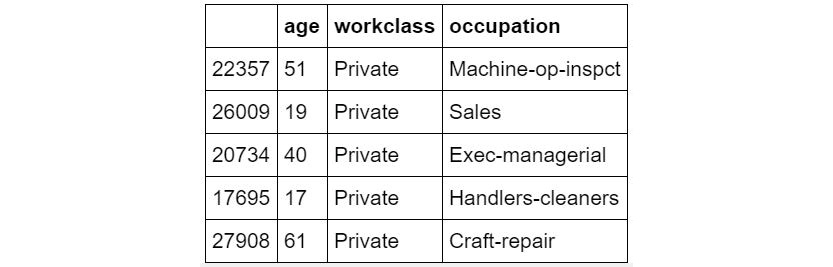
Figure 4.89: Output after merging the common keys
The second dataset is as follows:
df_2 = df[['education','occupation']].sample(5,random_state=101)
df_2.head()
The output is as follows:

Figure 4.90: Output after merging the common keys
- Merge the two datasets together:
df_merged = pd.merge(df_1,df_2,on='occupation',
how='inner').drop_duplicates()
df_merged
The output is as follows:
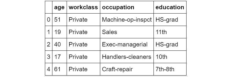
Figure 4.91: Output of distinct occupation values
Note
To access the source code for this specific section, please refer to https://packt.live/37IamwR.
You can also run this example online at https://packt.live/2YhuF1j.
5. Getting Comfortable with Different Kinds of Data Sources
Activity 5.01: Reading Tabular Data from a Web Page and Creating DataFrames
Solution:
These are the steps to complete this activity:
- Import BeautifulSoup and load the data by using the following command:
from bs4 import BeautifulSoup
import pandas as pd
- Open the Wikipedia file by using the following command:
fd = open("../datasets/List of countries by GDP (nominal) "
"- Wikipedia.htm", "r", encoding = "utf-8")
soup = BeautifulSoup(fd)
fd.close()
Note
Don't forget to change the path of the dataset (highlighted) based on its location on your system
- Calculate the tables by using the following command:
all_tables = soup.find_all("table")
print("Total number of tables are {} ".format(len(all_tables)))
There are nine tables in total.
- Find the right table using the class attribute by using the following command:
data_table = soup.find("table", {"class": '"wikitable"|}'})
print(type(data_table))
The output is as follows:
<class 'bs4.element.Tag'>
- Separate the source and the actual data by using the following command:
sources = data_table.tbody.findAll('tr', recursive=False)[0]
sources_list = [td for td in sources.findAll('td')]
print(len(sources_list))
The output is as follows:
3
- Use the findAll function to find the data from the body tag of data_table using the following command:
data = data_table.tbody.findAll('tr', recursive=False)[1]
.findAll('td', recursive=False)
- Use the findAll function to find the data from the data_table td tag by using the following command:
data_tables = []
for td in data:
data_tables.append(td.findAll('table'))
- Find the length of data_tables by using the following command:
len(data_tables)
The output is as follows:
3
- Check how to get the source names by using the following command:
source_names = [source.findAll('a')[0].getText()
for source in sources_list]
print(source_names)
The output is as follows:
['International Monetary Fund', 'World Bank', 'United Nations']
- Separate the header and data for the first source:
header1 = [th.getText().strip() for th in
data_tables[0][0].findAll('thead')[0].findAll('th')]
header1
The output is as follows:
['Rank', 'Country', 'GDP(US$MM)']
- Find the rows from data_tables using findAll:
rows1 = data_tables[0][0].findAll('tbody')[0].findAll('tr')[1:]
- Find the data from rows1 using the strip function for each td tag:
data_rows1 = [[td.get_text().strip() for td in
tr.findAll('td')] for tr in rows1]
- Find the DataFrame:
df1 = pd.DataFrame(data_rows1, columns=header1)
df1.head()
The output is as follows:
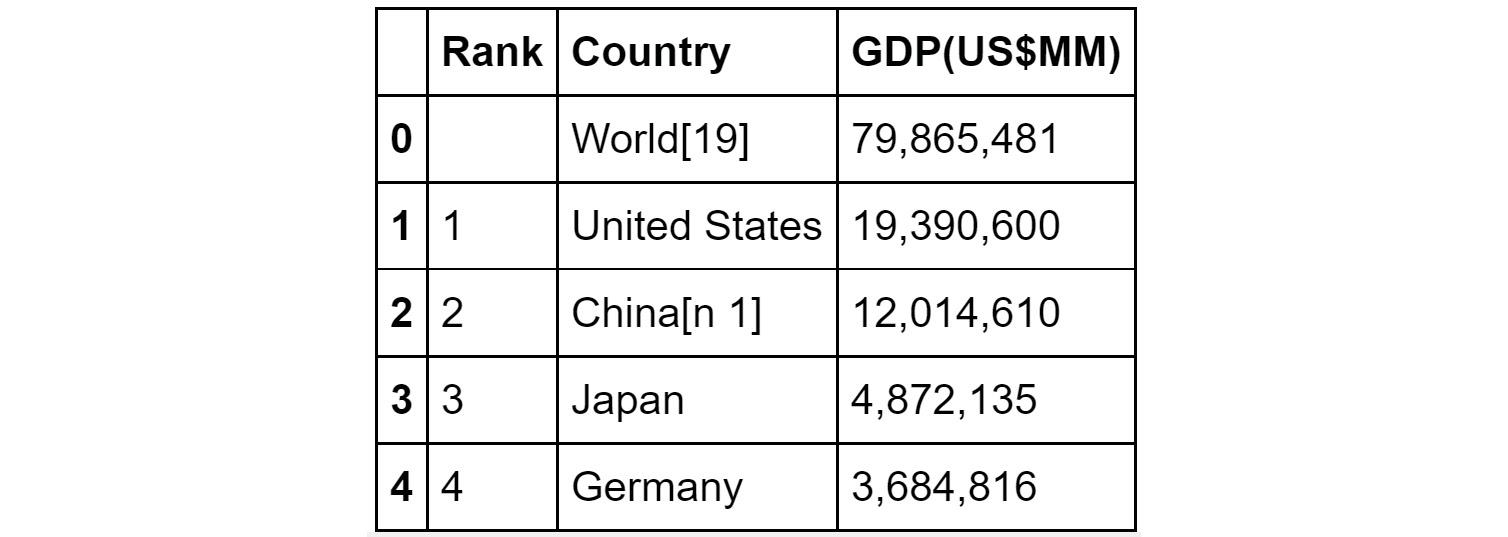
Figure 5.35: DataFrame created from the web page
- Do the same for the other two sources by using the following command:
header2 = [th.getText().strip() for th in data_tables[1][0]
.findAll('thead')[0].findAll('th')]
header2
The output is as follows:
['Rank', 'Country', 'GDP(US$MM)']
- Find the rows from data_tables using findAll by using the following command:
rows2 = data_tables[1][0].findAll('tbody')[0].findAll('tr')
- Define find_right_text using the strip function by using the following command:
def find_right_text(i, td):
if i == 0:
return td.getText().strip()
elif i == 1:
return td.getText().strip()
else:
index = td.text.find("♠")
return td.text[index+1:].strip()
- Find the rows from data_rows using find_right_text by using the following command:
data_rows2 = [[find_right_text(i, td) for i, td in
enumerate(tr.findAll('td'))] for tr in rows2]
- Calculate the df2 DataFrame by using the following command:
df2 = pd.DataFrame(data_rows2, columns=header2)
df2.head()
The output is as follows:
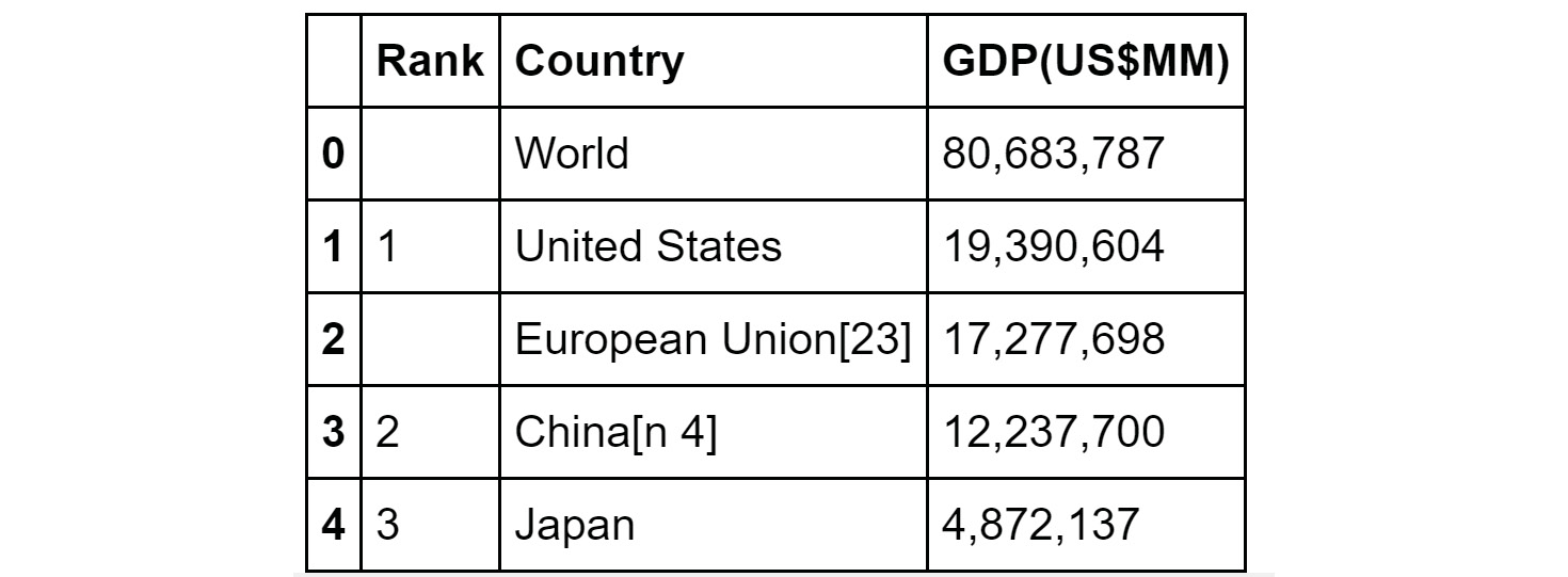
Figure 5.36: Output of the DataFrame
- Now, perform the same operations for the third DataFrame by using the following command:
header3 = [th.getText().strip() for th in data_tables[2][0]
.findAll('thead')[0].findAll('th')]
header3
The output is as follows:
['Rank', 'Country', 'GDP(US$MM)']
- Find the rows from data_tables using findAll by using the following command:
rows3 = data_tables[2][0].findAll('tbody')[0].findAll('tr')
- Find the rows from data_rows3 by using find_right_text:
data_rows3 = [[find_right_text(i, td) for i, td in
enumerate(tr.findAll('td'))] for tr in rows2]
- Calculate the df3 DataFrame by using the following command:
df3 = pd.DataFrame(data_rows3, columns=header3)
df3.head()
The output is as follows:
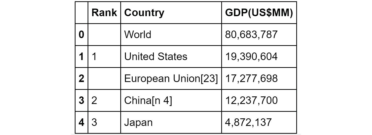
Figure 5.37: The third DataFrame
Note
To access the source code for this specific section, please refer to https://packt.live/2NaCrDB.
You can also run this example online at https://packt.live/2YRAukP.
6. Learning the Hidden Secrets of Data Wrangling
Activity 6.01: Handling Outliers and Missing Data
Solution:
The steps to completing this activity are as follows:
Note
The dataset to be used for this activity can be found at https://packt.live/2YajrLJ.
- Load the data:
import pandas as pd
import numpy as np
import matplotlib.pyplot as plt
%matplotlib inline
- Read the .csv file:
df = pd.read_csv("../datasets/visit_data.csv")
Note
Don't forget to change the path (highlighted) based on where the CSV file is saved on your system.
- Print the data from the DataFrame:
df.head()
The output is as follows:
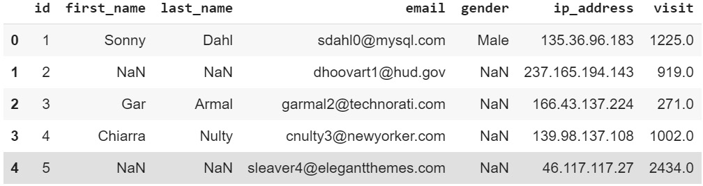
Figure 6.11: The contents of the CSV file
As we can see, there is data where some values are missing, and if we examine this, we will see some outliers.
- Check for duplicates by using the following command:
print("First name is duplicated - {}"
.format(any(df.first_name.duplicated())))
print("Last name is duplicated - {}"
.format(any(df.last_name.duplicated())))
print("Email is duplicated - {}"
.format(any(df.email.duplicated())))
The output is as follows:
First name is duplicated - True
Last name is duplicated - True
Email is duplicated - False
There are duplicates in both the first and last names, which is normal. However, as we can see, there are no duplicates in email. That's good.
- Check whether any essential column contains NaN:
"""
Notice that we have different ways to
format boolean values for the % operator
"""
print("The column Email contains NaN - %r " %
df.email.isnull().values.any())
print("The column IP Address contains NaN - %s " %
df.ip_address.isnull().values.any())
print("The column Visit contains NaN - %s " %
df.visit.isnull().values.any())
The output is as follows:
The column Email contains NaN - False
The column IP Address contains NaN - False
The column Visit contains NaN - True
The Visit column contains some NaN values. Given that the final task at hand will probably be predicting the number of visits, we cannot do anything with rows that do not have that information. They are a type of outlier. Let's get rid of them.
- Get rid of the outliers:
"""
There are various ways to do this. This is just one way. We encourage you to explore other ways. But before that we need to store the previous size of the data set and we will compare it with the new size
"""
size_prev = df.shape
df = df[np.isfinite(df['visit'])]
#This is an inplace operation.
# After this operation the original DataFrame is lost.
size_after = df.shape
- Report the size difference:
# Notice how parameterized format is used.
# Then, the indexing is working inside the quote marks
print("The size of previous data was - {prev[0]} rows and "
"the size of the new one is - {after[0]} rows"
.format(prev=size_prev, after=size_after))
The output is as follows:
The size of previous data was - 1000 rows and the size of the new one is - 974 rows
- Plot a box plot to find whether the data has outliers:
plt.boxplot(df.visit, notch=True)
The box plot is as follows:
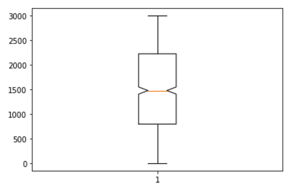
Figure 6.12: Box plot using the data
As we can see, we have data in this column in the interval (0, 3000). However, the main concentration of the data is between ~700 and ~2300.
- Get rid of values beyond 2900 and below 100 – these are outliers for us. We need to get rid of them:
df1 = df[(df['visit'] <= 2900) & (df['visit'] >= 100)]
# Notice the powerful & operator
"""
Here we abuse the fact the
number of variable can be greater
than the number of replacement targets
"""
print("After getting rid of outliers the new size of the data "
"is - {}".format(*df1.shape))
The output is as follows:
After getting rid of outliers the new size of the data is - 923
Note
To access the source code for this specific section, please refer to https://packt.live/2AFcSbn.
You can also run this example online at https://packt.live/3fAL9qY
7. Advanced Web Scraping and Data Gathering
Activity 7.01: Extracting the Top 100 e-books from Gutenberg
Solution:
These are the steps to complete this activity:
- Import the necessary libraries, including regex and BeautifulSoup:
import urllib.request, urllib.parse, urllib.error
import requests
from bs4 import BeautifulSoup
import ssl
import re
- Read the HTML from the URL:
top100url = 'https://www.gutenberg.org/browse/scores/top'
response = requests.get(top100url)
- Write a small function to check the status of the web request:
def status_check(r):
if r.status_code==200:
print("Success!")
return 1
else:
print("Failed!")
return -1
- Check the status of response:
status_check(response)
The output is as follows:
Success!
1
- Decode the response and pass it on to BeautifulSoup for HTML parsing:
contents = response.content.decode(response.encoding)
soup = BeautifulSoup(contents, 'html.parser')
- Find all the href tags and store them in the list of links.
# Empty list to hold all the http links in the HTML page
lst_links=[]
# Find all href tags and store them in the list of links
for link in soup.find_all('a'):
#print(link.get('href'))
lst_links.append(link.get('href'))
- Check what the list looks like – print the first 30 elements:
lst_links[:30]
The output (partially shown) is as follows:
['/wiki/Main_Page',
'/catalog/',
'/ebooks/',
'/browse/recent/last1',
'/browse/scores/top',
'/wiki/Gutenberg:Offline_Catalogs',
'/catalog/world/mybookmarks',
'/wiki/Main_Page',
'https://www.paypal.com/xclick/business=donate%40gutenberg.org&item_name=Donation+to+Project+Gutenberg',
'/wiki/Gutenberg:Project_Gutenberg_Needs_Your_Donation',
'http://www.ibiblio.org',
'http://www.pgdp.net/',
'pretty-pictures',
'#books-last1',
'#authors-last1',
'#books-last7',
'#authors-last7',
'#books-last30',
'#authors-last30',
'/ebooks/1342',
'/ebooks/84',
'/ebooks/1080',
'/ebooks/46',
'/ebooks/219',
'/ebooks/2542',
'/ebooks/98',
'/ebooks/345',
'/ebooks/2701',
'/ebooks/844',
'/ebooks/11']
- Use a regular expression to find the numeric digits in these links. These are the file numbers for the top 100 books. Initialize the empty list to hold the file numbers:
booknum=[]
Numbers 19 to 118 in the original list of links have the top 100 eBooks' numbers.
- Loop over the appropriate range and use a regex to find the numeric digits in the link (href) string. Use the findall() method:
for i in range(19,119):
link=lst_links[i]
link=link.strip()
"""
Regular expression to find the numeric digits in the link (href) string
"""
n=re.findall('[0-9]+',link)
if len(n)==1:
# Append the filenumber casted as integer
booknum.append(int(n[0]))
- Print the file numbers:
print(" The file numbers for the top 100 ebooks",
"on Gutenberg are shown below "+"-"*70)
print(booknum)
The output is as follows:
The file numbers for the top 100 ebooks on Gutenberg are shown below
----------------------------------------------------------------------
[1342, 84, 1080, 46, 219, 2542, 98, 345, 2701, 844, 11, 5200,
43, 16328, 76, 74, 1952, 6130, 2591, 1661, 41, 174, 23, 1260,
1497, 408, 3207, 1400, 30254, 58271, 1232, 25344, 58269, 158,
44881, 1322, 205, 2554, 1184, 2600, 120, 16, 58276, 5740, 34901,
28054, 829, 33, 2814, 4300, 100, 55, 160, 1404, 786, 58267, 3600,
19942, 8800, 514, 244, 2500, 2852, 135, 768, 58263, 1251, 3825,
779, 58262, 203, 730, 20203, 35, 1250, 45, 161, 30360, 7370,
58274, 209, 27827, 58256, 33283, 4363, 375, 996, 58270, 521,
58268, 36, 815, 1934, 3296, 58279, 105, 2148, 932, 1064, 13415]
Note
Since the list of top 100 books is frequently updated, the output you get will vary.
What does the soup object's text look like?
- Use the .text method and print only the first 2,000 characters (do not print the whole thing as it is too long).
You will notice a lot of empty spaces/blanks here and there. Ignore them. They are part of the HTML page's markup and its whimsical nature:
print(soup.text[:2000])
The output is as follows:
if (top != self) {
top.location.replace (http://www.gutenberg.org);
alert ('Project Gutenberg is a FREE service with NO membership required. If you paid somebody else to get here, make them give you your money back!');
}
Top 100 - Project Gutenberg
Online Book Catalog
Book Search
-- Recent Books
-- Top 100
-- Offline Catalogs
-- My Bookmarks
Main Page
…
Pretty Pictures
Top 100 EBooks yesterday —
Top 100 Authors yesterday —
Top 100 EBooks last 7 days —
Top 100 Authors last 7 days —
Top 100 EBooks last 30 days —
Top 100 Authors last 30 days
Top 100 EBooks yesterday
Pride and Prejudice by Jane Austen (1826)
Frankenstein; Or, The Modern Prometheus by Mary Wollstonecraft Shelley (1367)
A Modest Proposal by Jonathan Swift (1020)
A Christmas Carol in Prose; Being a Ghost Story of Christmas by Charles Dickens (953)
Heart of Darkness by Joseph Conrad (887)
Et dukkehjem. English by Henrik Ibsen (761)
A Tale of Two Cities by Charles Dickens (741)
Dracula by Bram Stoker (732)
Moby Dick; Or, The Whale by Herman Melville (651)
The Importance of Being Earnest: A Trivial Comedy for Serious People by Oscar Wilde (646)
Alice's Adventures in Wonderland by Lewis Carrol
- Search the extracted text (using regex) from the soup object to find the names of the top 100 eBooks (yesterday's ranking):
lst_titles_temp=[]
- Create a starting index. It should point at the text Top 100 Ebooks yesterday. Use the splitlines method of soup.text. It splits the lines of the text of the soup object:
start_idx=soup.text.splitlines().index('Top 100 EBooks yesterday')
Note
Since the list of top 100 books is frequently updated, the output you get will vary.
- Run the for loop from 1-100 to add the strings of the next 100 lines to this temporary list. Hint: use the splitlines method:
for i in range(100):
lst_titles_temp.append(soup.text.splitlines()[start_idx+2+i])
- Use regex to extract only text from the name strings and append them to an empty list. Use match and span to find the indices and use them:
lst_titles=[]
for i in range(100):
id1,id2=re.match('^[a-zA-Z ]*',lst_titles_temp[i]).span()
lst_titles.append(lst_titles_temp[i][id1:id2])
- Print the list of titles:
for l in lst_titles:
print(l)
The partial output is as follows:
Pride and Prejudice by Jane Austen
Frankenstein
A Modest Proposal by Jonathan Swift
A Christmas Carol in Prose
Heart of Darkness by Joseph Conrad
Et dukkehjem
A Tale of Two Cities by Charles Dickens
Dracula by Bram Stoker
Moby Dick
The Importance of Being Earnest
Alice
Metamorphosis by Franz Kafka
The Strange Case of Dr
Beowulf
…
The Russian Army and the Japanese War
Calculus Made Easy by Silvanus P
Beyond Good and Evil by Friedrich Wilhelm Nietzsche
An Occurrence at Owl Creek Bridge by Ambrose Bierce
Don Quixote by Miguel de Cervantes Saavedra
Blue Jackets by Edward Greey
The Life and Adventures of Robinson Crusoe by Daniel Defoe
The Waterloo Campaign
The War of the Worlds by H
Democracy in America
Songs of Innocence
The Confessions of St
Modern French Masters by Marie Van Vorst
Persuasion by Jane Austen
The Works of Edgar Allan Poe
The Fall of the House of Usher by Edgar Allan Poe
The Masque of the Red Death by Edgar Allan Poe
The Lady with the Dog and Other Stories by Anton Pavlovich Chekhov
Note
Since the list of top 100 books is frequently updated, the output you get will vary.
Here, we have seen how we can use web scraping and parsing using a mix of BeautifulSoup and regex to find information from very untidy and vast source data. These are some essential steps that you will have to perform on a daily basis when you are dealing with data wrangling.
Note
To access the source code for this specific section, please refer to https://packt.live/2BltmFo.
You can also run this example online at https://packt.live/37FdLwD.
Activity 7.02: Building Your Own Movie Database by Reading an API
SOLUTION
Note
Before you begin, ensure that you modify the APIkeys.json file and add your secret API key there. Link to the file: https://packt.live/2CmIpze.
These are the steps to complete this activity:
- Import urllib.request, urllib.parse, urllib.error, and json:
import urllib.request, urllib.parse, urllib.error
import json
- Load the secret API key (you have to get one from the OMDb website and use that; it has a daily API key limit of 1,000) from a JSON file, stored in the same folder, into a variable, by using json.loads():
Note
The following cell will not be executed in the solution notebook because the author cannot give out their private API key.
The students/users will need to obtain a key and store it in a JSON file. We are calling this file APIkeys.json.
- Open the APIkeys.json file by using the following command:
with open('APIkeys.json') as f:
keys = json.load(f)
omdbapi = keys['OMDBapi']
The final URL to be passed should look like this: http://www.omdbapi.com/?t=movie_name&apikey=secretapikey.
- Assign the OMDb portal (http://www.omdbapi.com/?) as a string to a variable called serviceurl by using the following command:
serviceurl = 'http://www.omdbapi.com/?'
- Create a variable called apikey with the last portion of the URL (&apikey=secretapikey), where secretapikey is your own API key. The movie name portion is t=movie_name, and it will be addressed later:
apikey = '&apikey='+omdbapi
- Write a utility function called print_json to print the movie data from a JSON file (which we will get from the portal). Here are the keys of a JSON file: 'Title', 'Year', 'Rated', 'Released', 'Runtime', 'Genre', 'Director', 'Writer', 'Actors', 'Plot', 'Language','Country', 'Awards', 'Ratings', 'Metascore', 'imdbRating', 'imdbVotes', and 'imdbID':
def print_json(json_data):
list_keys = ['Title', 'Year', 'Rated', 'Released',
'Runtime', 'Genre', 'Director', 'Writer',
'Actors', 'Plot', 'Language', 'Country',
'Awards', 'Ratings','Metascore', 'imdbRating',
'imdbVotes', 'imdbID']
print("-"*50)
for k in list_keys:
if k in list(json_data.keys()):
print(f"{k}: {json_data[k]}")
print("-"*50)
- Write a utility function to download a poster of the movie based on the information from the JSON dataset and save it in your local folder. Use the os module. The poster data is stored in the JSON key Poster. You may want to split the name of the Poster file and extract the file extension only. Let's say that the extension is .jpg. We could later join this extension to the movie name and create a filename such as movie.jpg. Use the open Python command open to open a file and write the poster data. Close the file after you're done. This function may not return anything. It just saves the poster data as an image file:
def save_poster(json_data):
import os
title = json_data['Title']
poster_url = json_data['Poster']
"""
Splits the poster url by '.' and
picks up the last string as file extension
"""
poster_file_extension=poster_url.split('.')[-1]
# Reads the image file from web
poster_data = urllib.request.urlopen(poster_url).read()
savelocation=os.getcwd()+''+'Posters'+''
"""
Creates new directory if the directory does not exist.
Otherwise, just use the existing path.
"""
if not os.path.isdir(savelocation):
os.mkdir(savelocation)
filename=savelocation+str(title)
+'.'+poster_file_extension
f=open(filename,'wb')
f.write(poster_data)
f.close()
- Write a utility function called search_movie to search a movie by its name, print the downloaded JSON data (use the print_json function for this), and save the movie poster in the local folder (use the save_poster function for this). Use a try-except loop for this, that is, try to connect to the web portal. If successful, proceed, but if not (that is, if an exception is raised), then just print an error message. Use the previously created variables, serviceurl and apikey. You have to pass on a dictionary with a key, t, and the movie name as the corresponding value to the urllib.parse.urlencode function and then add the serviceurl and apikey variables to the output of the function to construct the full URL. This URL will be used to access the data. The JSON data has a key called Response. If it is True, that means that the read was successful. Check this before processing the data. If it was not successful, then print the JSON key Error, which will contain the appropriate error message that's returned by the movie database:
def search_movie(title):
try:
url = serviceurl
+ urllib.parse.urlencode({'t':str(title)})+apikey
print(f'Retrieving the data of "{title}" now... ')
print(url)
uh = urllib.request.urlopen(url)
data = uh.read()
json_data=json.loads(data)
if json_data['Response']=='True':
print_json(json_data)
"""
Asks user whether to download the poster of the movie
"""
if json_data['Poster']!='N/A':
save_poster(json_data)
else:
print("Error encountered: ", json_data['Error'])
except urllib.error.URLError as e:
print(f"ERROR: {e.reason}")
- Test the search_movie function by entering Titanic:
search_movie("Titanic")
The following is the retrieved data for Titanic:
http://www.omdbapi.com/?t=Titanic&apikey=<your api key>
--------------------------------------------------
Title: Titanic
Year: 1997
Rated: PG-13
Released: 19 Dec 1997
Runtime: 194 min
Genre: Drama, Romance
Director: James Cameron
Writer: James Cameron
Actors: Leonardo DiCaprio, Kate Winslet, Billy Zane, Kathy Bates
Plot: A seventeen-year-old aristocrat falls in love with a kind but poor artist aboard the luxurious, ill-fated R.M.S. Titanic.
Language: English, Swedish
Country: USA
Awards: Won 11 Oscars. Another 111 wins & 77 nominations.
Ratings: [{'Source': 'Internet Movie Database', 'Value': '7.8/10'}, {'Source': 'Rotten Tomatoes', 'Value': '89%'}, {'Source': 'Metacritic', 'Value': '75/100'}]
Metascore: 75
imdbRating: 7.8
imdbVotes: 913,780
imdbID: tt0120338
--------------------------------------------------
- Test the search_movie function by entering Random_error (obviously, this will not be found, and you should be able to check whether your error-catching code is working properly):
search_movie("Random_error")
Retrieve the data of Random_error:
Retrieving the data of "Random_error" now...
http://www.omdbapi.com/?t=Random_error&apikey=<your api key>
Error encountered: Movie not found!
Note
In the last two steps, we've not shown the private API key (highlighted) for security reasons.
To access the source code for this specific section, please refer to https://packt.live/3hLJvoy.
You can also run this example online at https://packt.live/3efkDTZ.
8. RDBMS and SQL
Activity 8.01: Retrieving Data Accurately from Databases
Solution:
These are the steps to complete this activity:
- Connect to the supplied petsdb database:
import sqlite3
conn = sqlite3.connect("petsdb")
- Write a function to check whether the connection has been successful:
# a tiny function to make sure the connection is successful
def is_opened(conn):
try:
conn.execute("SELECT * FROM persons LIMIT 1")
return True
except sqlite3.ProgrammingError as e:
print("Connection closed {}".format(e))
return False
print(is_opened(conn))
The output is as follows:
True
- Close the connection:
conn.close()
- Check whether the connection is open or closed:
print(is_opened(conn))
The output is as follows:
Connection closed Cannot operate on a closed database.
False
- Connect to the petsdb database:
conn = sqlite3.connect("petsdb")
c = conn.cursor()
- Find out the different age groups in the persons table. Execute the following command:
for ppl, age in c.execute("SELECT count(*),
age FROM persons GROUP BY age"):
print("We have {} people aged {}".format(ppl, age))
The output is as follows:
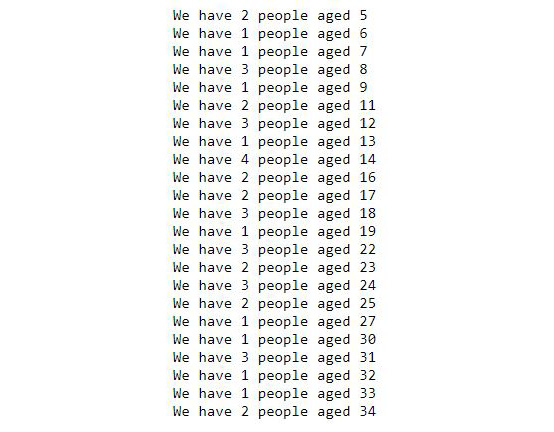
Figure 8.13: Section of output grouped by age
- To find out which age group has the maximum number of people, execute the following command:
for ppl, age in c.execute("SELECT count(*), age FROM persons
GROUP BY age ORDER BY count(*)DESC"):
print("The highest number of people is {} and "
"came from {} age group".format(ppl, age))
break
The output is as follows:
The highest number of people is 5 and came from 73 age group
- To find out how many people do not have a full name (the last name is blank/null), execute the following command:
res = c.execute("SELECT count(*) FROM persons
WHERE last_name IS null")
for row in res:
print(row)
The output is as follows:
(60,)
- To find out how many people have more than one pet, execute the following command:
res = c.execute("SELECT count(*) FROM
(SELECT count(owner_id) FROM pets
GROUP BY owner_id HAVING count(owner_id) >1)")
for row in res:
print("{} people have more than one pets".format(row[0]))
The output is as follows:
43 People have more than one pets
- To find out how many pets have received treatment, execute the following command:
res = c.execute("SELECT count(*) FROM pets
WHERE treatment_done=1")
for row in res:
print(row)
The output is as follows:
(36,)
- To find out how many pets have received treatment and the type of pet is known, execute the following command:
res = c.execute("SELECT count(*) FROM pets
WHERE treatment_done=1 AND pet_type IS NOT null")
for row in res:
print(row)
The output is as follows:
(16,)
- To find out how many pets are from the city called east port, execute the following command:
res = c.execute("SELECT count(*) FROM pets
JOIN persons ON pets.owner_id = persons.id
WHERE persons.city='east port'")
for row in res:
print(row)
The output is as follows:
(49,)
- To find out how many pets are from the city called east port and who received treatment, execute the following command:
res = c.execute("SELECT count(*) FROM pets
JOIN persons ON pets.owner_id =
persons.id WHERE persons.city='east port'
AND pets.treatment_done=1")
for row in res:
print(row)
The output is as follows:
(11,)
Note
To access the source code for this specific section, please refer to https://packt.live/3derN9D.
You can also run this example online at https://packt.live/2ASWYKi.
9. Applications in Business Use Cases and Conclusion of the Course
Activity 9.01: Data Wrangling Task – Fixing UN Data
Solution:
These are the steps to complete this activity:
- Import the required libraries:
import numpy as np
import pandas as pd
import matplotlib.pyplot as plt
import warnings
warnings.filterwarnings('ignore')
- Save the URL of the dataset (highlighted) and use the pandas read_csv method to directly pass this link and create a DataFrame:
education_data_link="http://data.un.org/_Docs/SYB/CSV/"
"SYB61_T07_Education.csv"
df1 = pd.read_csv(education_data_link)
- Print the data in the DataFrame:
df1.head()
The output (partially shown) is as follows:
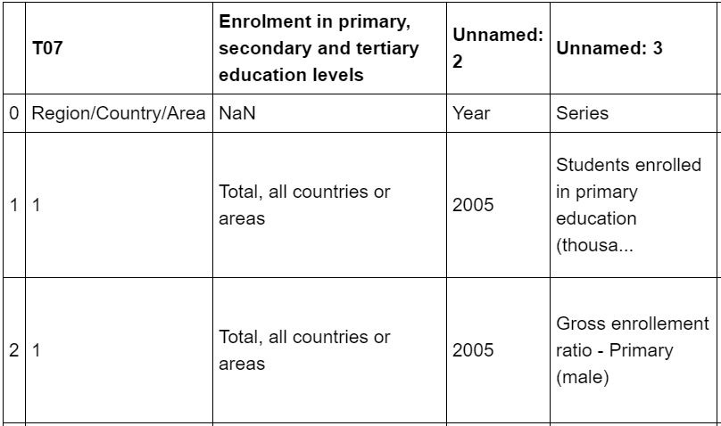
Figure 9.7: Partial DataFrame from the UN data
- As the first row does not contain useful information, use the skiprows parameter to remove the first row:
df1 = pd.read_csv(education_data_link,skiprows=1)
- Print the data in the DataFrame:
df1.head()
The output is as follows:
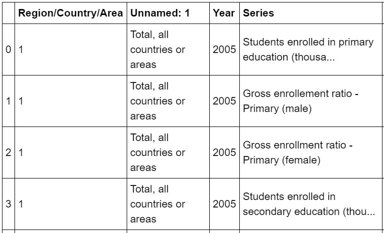
Figure 9.8: Partial DataFrame after removing the first row
- Drop the Region/Country/Area and Source columns as they will not be very helpful:
df2 = df1.drop(['Region/Country/Area','Source'],axis=1)
- Assign the following names as the columns of the DataFrame: ['Region/Country/Area','Year','Data','Value','Footnotes']
df2.columns=['Region/Country/Area','Year','Data',
'Enrollments (Thousands)','Footnotes']
- Print the data in the DataFrame:
df2.head()
The output is as follows:
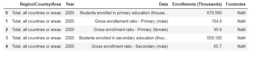
Figure 9.9: DataFrame after dropping the Region/Country/Area and Source columns
- Check how many unique values the Footnotes column contains:
df2['Footnotes'].unique()
The output is as follows:

Figure 9.10: Unique values of the Footnotes column
- Convert the Value column data into a numeric one for further processing:
type(df2['Enrollments (Thousands)'][0])
The output is as follows:
str
- Create a utility function to convert the strings in the Value column into floating-point numbers:
def to_numeric(val):
"""
Converts a given string (with one or more commas) to a numeric value
"""
if ',' not in str(val):
result = float(val)
else:
val=str(val)
val=''.join(str(val).split(','))
result=float(val)
return result
- Use the apply method to apply this function to the Value column data:
df2['Enrollments (Thousands)']=df2['Enrollments (Thousands)']
.apply(to_numeric)
- Print the unique types of data in the Data column:
df2['Data'].unique()
The output is as follows:
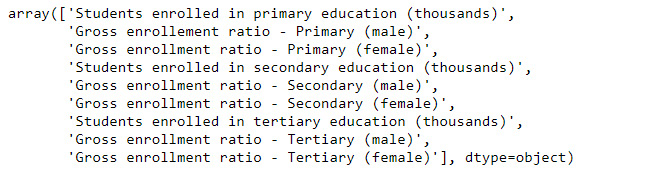
Figure 9.11: Unique values in a column
- Create three DataFrames by filtering and selecting them from the original DataFrame:
df_primary: Only students enrolled in primary education (thousands)
df_secondary: Only students enrolled in secondary education (thousands)
df_tertiary: Only students enrolled in tertiary education (thousands):
df_primary = df2[df2['Data']=='Students enrolled in primary '
'education (thousands)']
df_secondary = df2[df2['Data']=='Students enrolled in secondary '
'education (thousands)']
df_tertiary = df2[df2['Data']=='Students enrolled in tertiary '
'education (thousands)']
- Compare them using bar charts of the primary students' enrollment of a low-income country and a high-income country:
primary_enrollment_india = df_primary[df_primary
['Region/Country/Area']=='India']
primary_enrollment_USA = df_primary[df_primary
['Region/Country/Area']
=='United States of America']
- Print the primary_enrollment_india data:
primary_enrollment_india
The output is as follows:
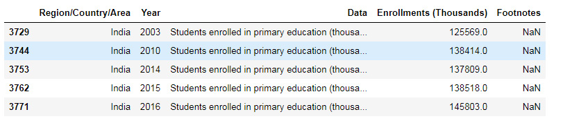
Figure 9.12: Data for enrollment in primary education in India
- Print the primary_enrollment_USA data:
primary_enrollment_USA
The output is as follows:
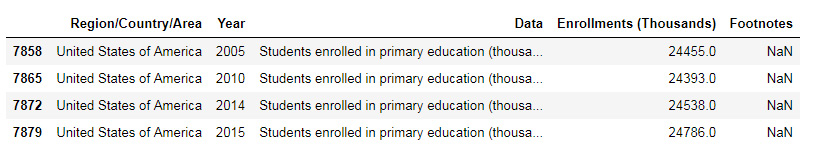
Figure 9.13: Data for enrollment in primary education in USA
- Plot the data for India:
plt.figure(figsize=(8,4))
plt.bar(primary_enrollment_india['Year'],
primary_enrollment_india['Enrollments (Thousands)'])
plt.title("Enrollment in primary education in India "
"(in thousands)",fontsize=16)
plt.grid(True)
plt.xticks(fontsize=14)
plt.yticks(fontsize=14)
plt.xlabel("Year", fontsize=15)
plt.show()
The output is as follows:
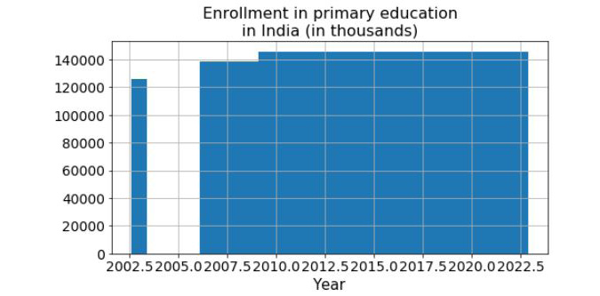
Figure 9.14: Bar plot for enrollment in primary education in India
- Plot the data for the USA:
plt.figure(figsize=(8,4))
plt.bar(primary_enrollment_USA['Year'],
primary_enrollment_USA['Enrollments (Thousands)'])
plt.title("Enrollment in primary education in the "
"United States of America (in thousands)",fontsize=16)
plt.grid(True)
plt.xticks(fontsize=14)
plt.yticks(fontsize=14)
plt.xlabel("Year", fontsize=15)
plt.show()
The output is as follows:
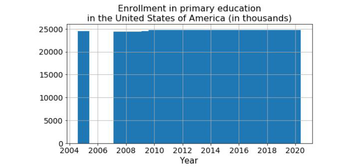
Figure 9.15: Bar plot for enrollment in primary education in the USA
As we can see, we have missing data. Now is the time to use pandas methods to do the data imputation. But to do that, we need to create a DataFrame with missing values inserted into it – that is, we need to append another DataFrame with missing values to the current DataFrame.
- Find the missing years:
missing_years = [y for y in range(2004,2010)]
+[y for y in range(2011,2014)]
- Print the value in the missing_years variable:
missing_years
The output is as follows:
[2004, 2005, 2006, 2007, 2008, 2009, 2011, 2012, 2013]
- Create a dictionary of values with np.nan. Note that there are nine missing data points, so we need to create a list with identical values repeated nine times:
dict_missing =
{'Region/Country/Area':['India']*9,
'Year':missing_years,
'Data':'Students enrolled in primary education(thousands)'*9,
'Enrollments (Thousands)':[np.nan]*9,'Footnotes':[np.nan]*9}
- Create a DataFrame of missing values (from the preceding dictionary) that we can append:
df_missing = pd.DataFrame(data=dict_missing)
- Append the new DataFrames to the previously existing ones:
primary_enrollment_india=primary_enrollment_india
.append(df_missing,ignore_index=True,
sort=True)
- Print the data in primary_enrollment_india:
primary_enrollment_india
The output is as follows:
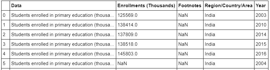
Figure 9.16: Partial Data for enrollment in primary education in India after appending the data
- Sort by year and reset the indices using reset_index. Use inplace=True to execute the changes on the DataFrame itself:
primary_enrollment_india.sort_values(by='Year',inplace=True)
primary_enrollment_india.reset_index(inplace=True,drop=True)
- Print the data in primary_enrollment_india:
primary_enrollment_india
The output is as follows:
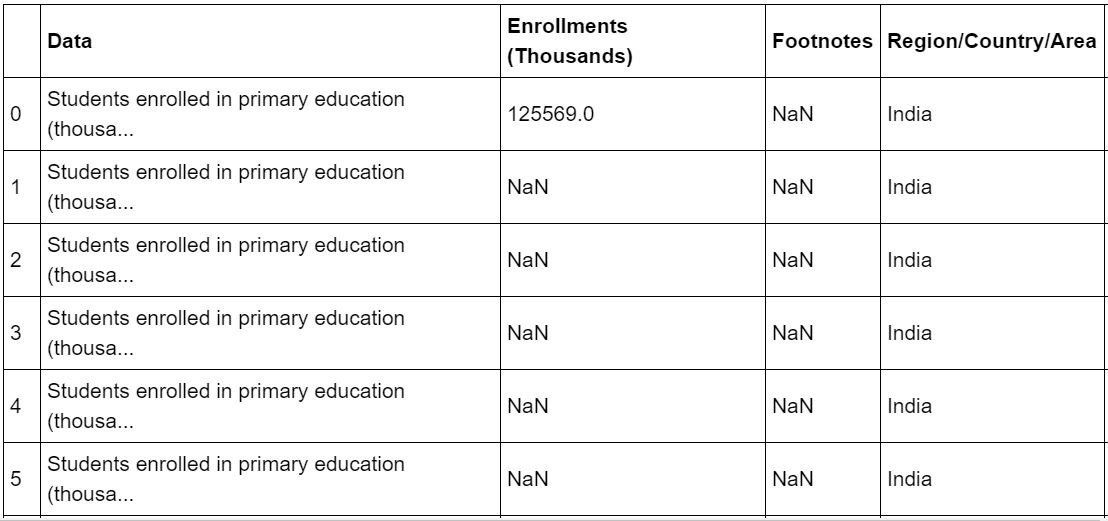
Figure 9.17: Partial Data for enrollment in primary education in India after sorting the data
- Use the interpolate method for linear interpolation. It fills all the NaN values with linearly interpolated values. Check out this link for more details about this method: http://pandas.pydata.org/pandas-docs/version/0.17/generated/pandas.DataFrame.interpolate.html:
primary_enrollment_india.interpolate(inplace=True)
- Print the data in primary_enrollment_india:
primary_enrollment_india
The output is as follows:
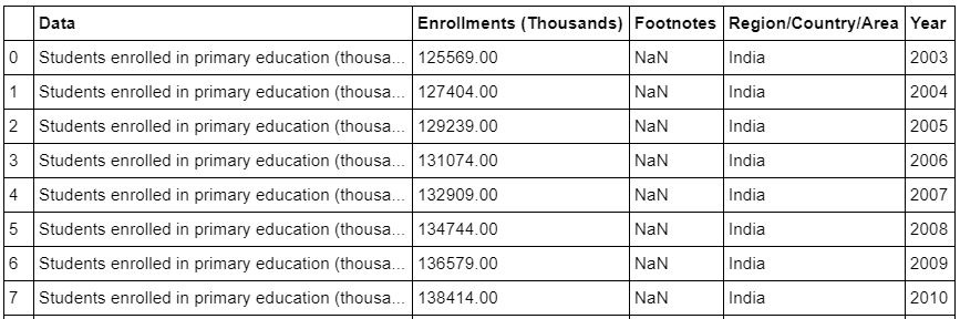
Figure 9.18: Data for enrollment in primary education in India after interpolating the data
- Plot the data:
plt.figure(figsize=(8,4))
plt.bar(primary_enrollment_india['Year'],
primary_enrollment_india['Enrollments (Thousands)'])
plt.title("Enrollment in primary education in India "
"(in thousands)", fontsize=16)
plt.grid(True)
plt.xticks(fontsize=14)
plt.yticks(fontsize=14)
plt.xlabel("Year", fontsize=15)
plt.show()
The output is as follows:
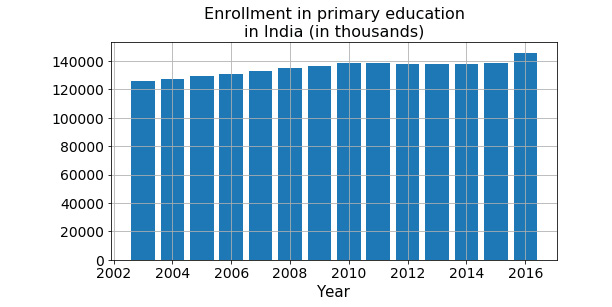
Figure 9.19: Bar plot for enrollment in primary education in India
- Repeat the same steps for the USA:
missing_years = [2004]+[y for y in range(2006,2010)]
+[y for y in range(2011,2014)]+[2016]
- Print the value in missing_years.
missing_years
The output is as follows:
[2004, 2006, 2007, 2008, 2009, 2011, 2012, 2013, 2016]
- Create dict_missing, as follows:
dict_missing =
{'Region/Country/Area':['United States of America']*9,
'Year':missing_years,
'Data':'Students enrolled in primary education (thousands)'*9,
'Value':[np.nan]*9,'Footnotes':[np.nan]*9}
- Create the DataFrame for df_missing, as follows:
df_missing = pd.DataFrame(data=dict_missing)
- Append this to the primary_enrollment_USA variable, as follows:
primary_enrollment_USA=primary_enrollment_USA
.append(df_missing,
ignore_index =True,sort=True)
- Sort the values in the primary_enrollment_USA variable, as follows:
primary_enrollment_USA.sort_values(by='Year',inplace=True)
- Reset the index of the primary_enrollment_USA variable, as follows:
primary_enrollment_USA.reset_index(inplace=True,drop=True)
- Interpolate the primary_enrollment_USA variable, as follows:
primary_enrollment_USA.interpolate(inplace=True)
- Print the primary_enrollment_USA variable:
primary_enrollment_USA
The output is as follows:
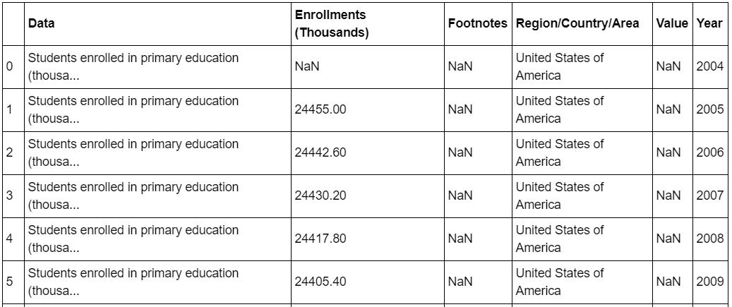
Figure 9.20: Data for enrollment in primary education in the USA after all operations have been completed
- Still, the first value is unfilled. We can use the limit and limit_direction parameters with the interpolate method to fill it in. How did we know this? By searching on Google and looking at the StackOverflow page. Always search for the solution to your problem and look for what has already been done and try to implement it:
primary_enrollment_USA.interpolate(method='linear',
limit_direction='backward',
limit=1)
The output is as follows:
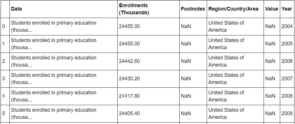
Figure 9.21: Data for enrollment in primary education in the USA after limiting the data
- Print the data in primary_enrollment_USA:
primary_enrollment_USA
The output is as follows:
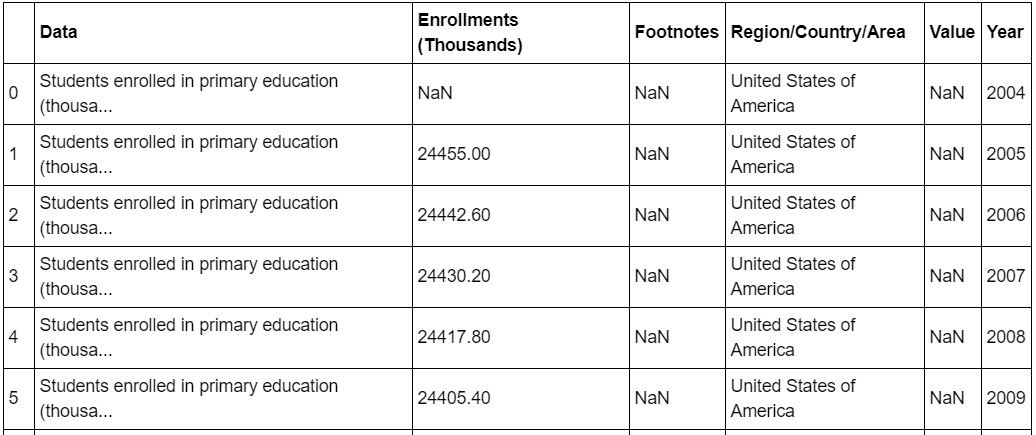
Figure 9.22: Data for enrollment in primary education in the USA
- Plot the data:
plt.figure(figsize=(8,4))
plt.bar(primary_enrollment_USA['Year'],
primary_enrollment_USA['Enrollments (Thousands)'])
plt.title("Enrollment in primary education in the "
"United States of America (in thousands)",fontsize=16)
plt.grid(True)
plt.xticks(fontsize=14)
plt.yticks(fontsize=14)
plt.xlabel("Year", fontsize=15)
plt.show()
The output is as follows:
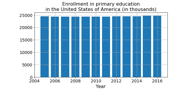
Figure 9.23: Bar plot for enrollment in primary education in the USA
Note
To access the source code for this specific section, please refer to https://packt.live/3fyIqy8.
You can also run this example online at https://packt.live/3fQ0PXJ.
Activity 9.02: Data Wrangling Task – Cleaning GDP Data
Solution:
These are the steps to complete this activity:
- Import the required libraries:
import numpy as np
import pandas as pd
import matplotlib.pyplot as plt
import warnings
warnings.filterwarnings('ignore')
- GDP data for India: We will try to read the GDP data for India from a CSV file that was found in a World Bank portal. It is given to you and also hosted on the Packt GitHub repository at https://packt.live/2AMoeu6. However, the pandas read_csv method will throw an error if we try to read it normally. Let's look at a step-by-step guide of how we can read useful information from it:
df3=pd.read_csv("../datasets/India_World_Bank_Info.csv")
Note
Throughout this activity, don't forget to change the path of the dataset (highlighted) to match its location on your system.
The output (partially shown) is as follows:
---------------------------------------------------------------------------
ParserError Traceback (most recent call last)
<ipython-input-45-9239cae67df7> in <module>()
...
ParserError: Error tokenizing data. C error: Expected 1 fields in line 6, saw 3
We can try and use the error_bad_lines=False option in this kind of situation.
- Read the India World Bank Information .csv file.
df3=pd.read_csv("../datasets/India_World_Bank_Info.csv",
error_bad_lines=False)
The output (partially shown) will be:
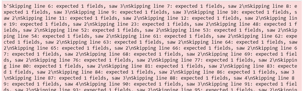
Figure 9.24: Partial output of the warnings.
- Then, let's take a look at the contents of the DataFrame.
df3.head(10)
The output is as follows:
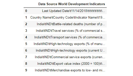
Figure 9.25: DataFrame from the India World Bank Information
Note
At times, the output may not be found because there are three rows instead of the expected one row.
- Clearly, the delimiter in this file is tab ( ):
df3=pd.read_csv("../datasets/India_World_Bank_Info.csv",
error_bad_lines=False,delimiter=' ')
df3.head(10)
The output is as follows:
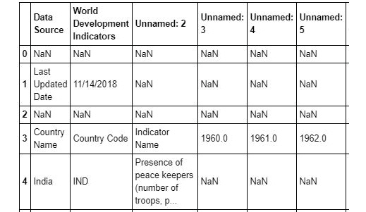
Figure 9.26: Partial output of the DataFrame from the India World Bank Information after using a delimiter
- Use the skiprows parameter to skip the first four rows:
df3=pd.read_csv("../datasets/India_World_Bank_Info.csv",
error_bad_lines=False,delimiter=' ',
skiprows=4)
df3.head(10)
The output is as follows:
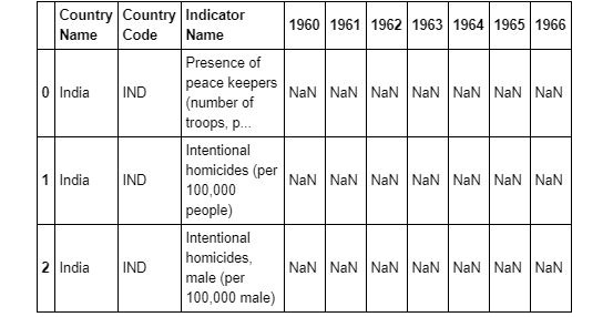
Figure 9.27: Partial output of DataFrame from the India World Bank Information after using skiprows
Closely examine the dataset. In this file, the columns are the yearly data and the rows are the various types of information. Upon examining the file with Excel, we find that the Indicator Name column is the one with the name of a particular data type, which is GDP per capita. We filter the dataset with the information we are interested in and also transpose (the rows and columns are interchanged) it to put it in a similar format to what our previous education dataset was in:
df4=df3[df3['Indicator Name']=='GDP per capita (current US$)'].T
df4.head(10)
The output is as follows:
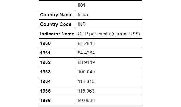
Figure 9.28: DataFrame focusing on GDP per capita
- There is no index, so let's use reset_index again:
df4.reset_index(inplace=True)
df4.head(10)
The output is as follows:
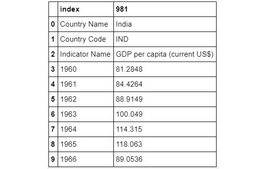
Figure 9.29: DataFrame from the India World Bank Information using reset_index
- The first three rows aren't useful. We can redefine the DataFrame without them. Then, we re-index again:
df4.drop([0,1,2],inplace=True)
df4.reset_index(inplace=True,drop=True)
df4.head(10)
The output is as follows:
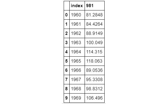
Figure 9.30: DataFrame from the India World Bank Information after dropping and resetting the index
- Let's rename the columns properly (this is necessary for merging, which we will look at shortly):
df4.columns=['Year','GDP']
df4.head(10)
The output is as follows:
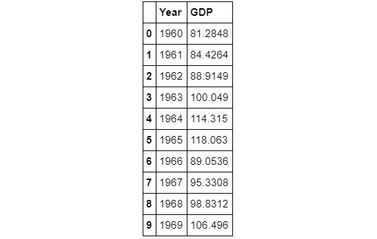
Figure 9.31: DataFrame focusing on Year and GDP
- It looks like we have GDP data from 1960 onward. However, we are only interested in 2003 – 2016. Let's examine the last 20 rows:
df4.tail(20)
The output is as follows:
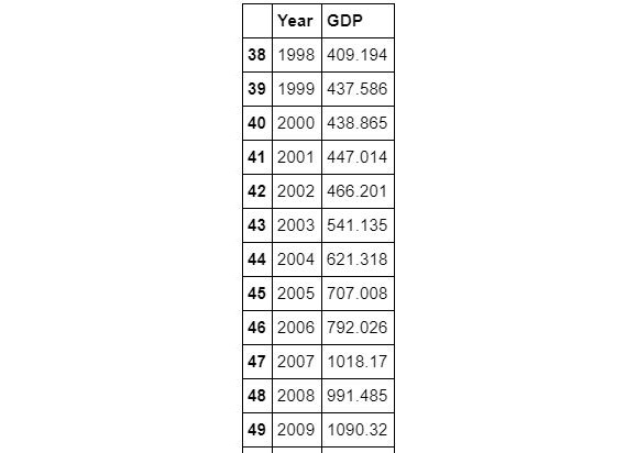
Figure 9.32: DataFrame from the India World Bank Information
- So, we should be good with rows 43-56. Let's create a DataFrame called df_gdp:
df_gdp=df4.iloc[[i for i in range(43,57)]]
df_gdp
The output is as follows:
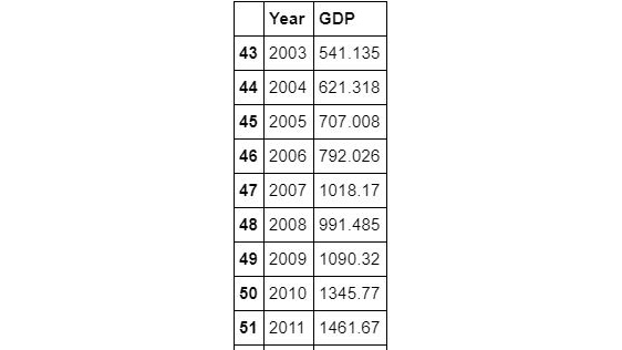
Figure 9.33: DataFrame from the India World Bank Information
- We need to reset the index again (for merging):
df_gdp.reset_index(inplace=True,drop=True)
df_gdp
The output is as follows:
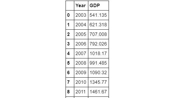
Figure 9.34: DataFrame from the India World Bank Information
- The year in this DataFrame is not of the int type. So, it will have problems merging with the education DataFrame:
df_gdp['Year']
The output is as follows:
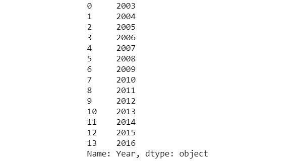
Figure 9.35: DataFrame focusing on year
- Use the apply method with Python's built-in int function. Ignore any warnings that are thrown:
df_gdp['Year']=df_gdp['Year'].apply(int)
Note
To access the source code for this specific section, please refer to https://packt.live/3fyIqy8.
You can also run this example online at https://packt.live/3fQ0PXJ.
Activity 9.03: Data Wrangling Task – Merging UN Data and GDP Data
These are the steps to complete this activity:
- Now, merge the two DataFrames, that is, primary_enrollment_india and df_gdp, on the Year column:
primary_enrollment_with_gdp=
primary_enrollment_india.merge(df_gdp,on='Year')
primary_enrollment_with_gdp
The output is as follows:
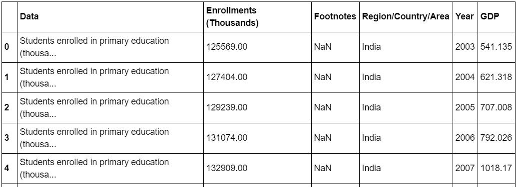
Figure 9.36: Merged data
- Now, we can drop the Data, Footnotes, and Region/Country/Area columns:
primary_enrollment_with_gdp.drop(['Data','Footnotes',
'Region/Country/Area'],
axis=1,inplace=True)
primary_enrollment_with_gdp
The output is as follows:
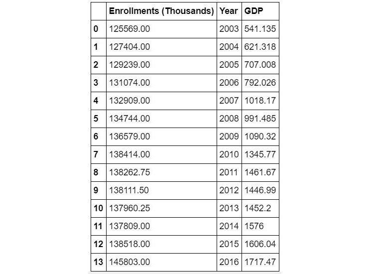
Figure 9.37: Merged data after dropping the Data, Footnotes, and Region/Country/Area columns
- Rearrange the columns for proper viewing and presentation to a data scientist:
primary_enrollment_with_gdp =
primary_enrollment_with_gdp[['Year',
'Enrollments (Thousands)','GDP']]
primary_enrollment_with_gdp
The output is as follows:
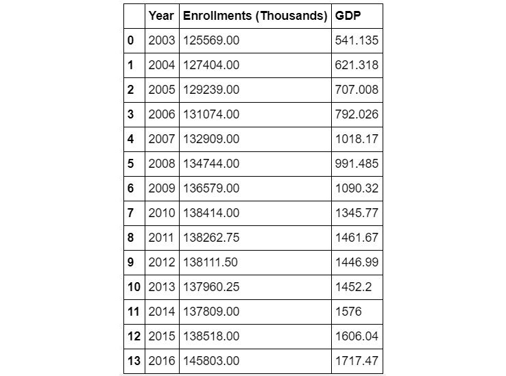
Figure 9.38: Merged data after rearranging the columns
- Plot the data:
plt.figure(figsize=(8,5))
plt.title("India's GDP per capita vs primary education "
"enrollment",fontsize=16)
plt.scatter(primary_enrollment_with_gdp['GDP'],
primary_enrollment_with_gdp['Enrollments (Thousands)'],
edgecolor='k',color='orange',s=200)
plt.xlabel("GDP per capita (US $)",fontsize=15)
plt.ylabel("Primary enrollment (thousands)", fontsize=15)
plt.xticks(fontsize=14)
plt.yticks(fontsize=14)
plt.grid(True)
plt.show()
The output is as follows:
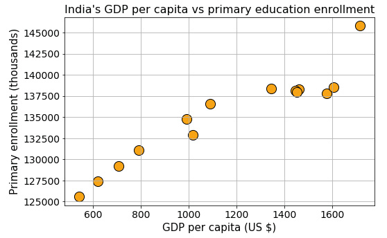
Figure 9.39: Scatter plot of merged data
Note
To access the source code for this specific section, please refer to https://packt.live/3fyIqy8.
You can also run this example online at https://packt.live/3fQ0PXJ.
Activity 9.04: Data Wrangling Task – Connecting the New Data to the Database
Solution:
These are the steps to complete this activity:
- Connect to a database and start writing values in it. We start by importing the sqlite3 module of Python and then use the connect function to connect to a database. Designate Year as the PRIMARY KEY of this table:
import sqlite3
with sqlite3.connect("Education_GDP.db") as conn:
cursor = conn.cursor()
cursor.execute("CREATE TABLE IF NOT EXISTS
education_gdp(Year INT, Enrollment
FLOAT, GDP FLOAT, PRIMARY KEY (Year))")
- Run a loop with the dataset rows one by one to insert them into the table:
with sqlite3.connect("Education_GDP.db") as conn:
cursor = conn.cursor()
for i in range(14):
year = int(primary_enrollment_with_gdp.iloc[i]['Year'])
enrollment =
primary_enrollment_with_gdp.iloc[i]
['Enrollments (Thousands)']
gdp = primary_enrollment_with_gdp.iloc[i]['GDP']
#print(year,enrollment,gdp)
cursor.execute("INSERT INTO
education_gdp (Year,Enrollment,GDP)
VALUES(?,?,?)",(year,enrollment,gdp))
If we look at the current folder, we should see a file called Education_GDP.db, and if we can examine that using a database viewer program, we will see that the data has been transferred there.
Note
To access the source code for this specific section, please refer to https://packt.live/3fyIqy8.
You can also run this example online at https://packt.live/3fQ0PXJ.