Machine learning has become a hot topic again recently mostly due to the high amount of data being generated and stored and also the improvement in processing capabilities. Machine learning algorithms are much more than a research topic; they are being used by companies as a competitive advantage. In this chapter, we will discuss the most famous machine learning algorithms focusing on artificial neural networks and show how JavaFX can be used along with a solid machine learning library, DeepLearning4J (DL4J). We will focus on visual neural network models that can interact directly with JavaFX.
What Is Machine Learning
When you develop a system, you have to program exactly what it is supposed to do. You develop an algorithm that step by step describes how a specific flow must be executed.
Machine learning techniques are different, since they don’t require explicit programming steps. These techniques return results without being explicitly programmed. Instead of programming it, you “teach” the machine how to use data.
In the machine learning world, we have two different types of algorithms for different tasks, with different performances and precisions. We divide these algorithms in two main categories:
Supervised learning
Unsupervised learning
Both categories require data as input.
Supervised Learning
In supervised learning, we have algorithms that make use of labeled data, which means that you will provide sample instances of a problem for the algorithm so it can learn how to classify new unlabeled instances of the same problem. For example, let’s say you have certain images of dogs and cats, and you use these images on some of the algorithms. After teaching the algorithm, you can input new images into it, and it should tell you if the new image contains a cat or a dog.
To teach the algorithm, you need to input information, a lot of information, and adjust the algorithm parameters until it can reasonably predict new data. This process is called training. Imagine you want to identify your family in photos and you have thousands of photos of your family members. Once these photos are correctly labeled, you can use them to feed an algorithm, and once the algorithm has a good precision, it can be used to predict new pictures, hopefully identifying members of your family!
Unsupervised Learning
When you have data that you don’t have further information about, but still you want to retrieve some knowledge from, you can use unsupervised learning; and depending on the chosen algorithm, it can group certain instances of your data. A known example for unsupervised learning is the recommendation system, where you use user data on certain systems to suggest to them other products or movies.
To use machine learning techniques, one can choose between multiple algorithms available. For supervised learning, we have regression, decision trees, and more. For unsupervised learning, you will find clustering, anomaly detection, and others. For supervised and unsupervised learning, we have neural networks, which we will explore in this chapter.
Artificial Neural Networks
Artificial neural networks are famous and highly discussed and researched due to the high amount of data available for training and high-performance CPUs and GPUs. Neural network basic elements are artificial neurons, which are based on “neurological neurons” and composed of input numbers (x) that are multiplied by their weight (w) and summed by a bias, and the result is inserted in an activation function. Then we have the result (y). These neurons are organized in layers that can have n neurons. Layers are connected in different architectures, and finally we have an artificial neural network as shown in Figure 13-1. Nowadays, artificial neural networks are composed of thousands of neurons, sometimes with hundreds of layers. These large artificial neural networks are part of deep learning methods, and we will see some of the famous deep neural network architectures in this chapter.
Figure 13-1
An example of a neural network
The training process is the key for a neural network to be useful. Before training, the neural network starts with random weights. Training consists of inputting data in the neural network, measuring how far it is from the actual information, and then adjusting the weights until the results are close to the actual values (also called ground truth). For example, if you have a neural network that can predict if a given image is a cat or a dog, you input a cat, and it returns that the cat has 80% of being a dog, you calculate an error (how far is the result from the ground truth data) and then use the process called backpropagation to adjust the neural network weights and repeat it with thousand images of cats and dogs until you have a good result. During training, you should be concerned about overfitting, but this is out of this book’s scope.
There are quite a few very known neural network architectures available for use, most of which were proposed by big companies or artificial intelligence researchers. You may create your own neural network, get a lot of data, and train it, so you can use it in your application; however, in this chapter, we will use pretrained neural networks. Yes, good souls out there got some of the very known neural network architectures, trained them using some known dataset (e.g., ImageNet), and, once they were trained, made them available for use in applications; these are called pretrained neural network models.
The power of a pretrained neural network is that it will have all weights already adjusted for a certain dataset, meaning that it is ready for use and you can adjust the weights again with your own data, making it ready to deal with new classes reusing knowledge from other images or data.
Convolutional Neural Networks
It is out of the scope of this book to go deep in all neural network architectures and techniques; however, since we will use mostly convolutional neural networks (CNNs), whose architecture is useful to detect patterns in images without having to write specific patterns, let’s discuss it. To understand how CNNs work, take as an example Figure 13-2, a bee drawn by my wife, in an application we will discuss later.
Figure 13-2
An example of an image to be analyzed by a CNN
Looking at this bee, we can identify some patterns: a wing is a curve, the body also has a few curves and a filled part, the head is an oval form, and so on. You probably don’t know how, but your brain identifies these patterns and concludes that this is a bee drawing. A CNN contains a convolutional layer used with pooling and normalization layers that can identify these patterns, and you don’t have to hard-code it. This is all learned during the training process.
The output of CNN layers is then passed on to a fully connected architecture, which will end in neurons representing each class of images (bee, frogs, dogs, etc.). When you actually predict an image, each class will have a percent chance of being of a certain class. See the following example where the CNN behind the application knows that we tried to input a mouse image (~78% of a mouse), but it also says that there’s a small chance that it is a lion (~13%) as shown in Figure 13-3!
Figure 13-3
The results of an image prediction performed by a CNN
Eclipse DeepLearning4J: Java API for Neural Networks
If you search for deep learning and Java, you will find a few libraries out there. For our purpose, we will use Eclipse DeepLearning4J (DL4J), which allows easy data vectorization, creation of neural networks, and training and offers pretrained models for immediate use and can run even on mobile devices.
The core library used by DL4J is ND4J. We can perform vectors of n-size operations with ND4J; hence, it is used in all neural network operations in DL4J. For example, every data you want to load for training or predictions is converted to an ND4J INDArray object, so it can feed a neural network during the training process. For more information about ND4J, see Chapter 14, “Scientific Applications Using JavaFX.”
On top of ND4J, we have the DataVec library. Deal with neural networks is deal with data, and data on a neural network is represented by number vectors of n size. You can’t simply input the binaries of an image or a text string into a neural network. You must convert it; and DataVec has all the tools to go through images, text, CSV files, and more into a neural network. Later, we will make use of DataSetIterators, and it will make clear how it is useful.
DeepLearning4J setup using Maven is simple; you have to add the nd4j-native-platform and deeplearning4j-core dependencies. For this chapter, we will also need deeplearning4j-zoo to make use of available neural network models. For this chapter, we use deeplearning4j 1.0.0-beta7:
<dependency>
<groupId>org.nd4j</groupId>
<artifactId>nd4j-native-platform</artifactId>
<version>${dl4j.version}</version>
</dependency>
<dependency>
<groupId>org.deeplearning4j</groupId>
<artifactId>deeplearning4j-core</artifactId>
<version>${dl4j.version}</version>
</dependency>
<dependency>
<groupId>org.deeplearning4j</groupId>
<artifactId>deeplearning4j-zoo</artifactId>
<version>${dl4j.version}</version>
</dependency>
We won’t be creating neural networks, but to have a taste of how neural networks are created with DeepLearning4J, it looks like you may check DeepLearning4J examples (https://github.com/eclipse/deeplearning4j-examples), like the version of LeNet (the first CNN architecture) that is available and will be used in the first JavaFX application from this chapter:
MultiLayerConfiguration conf = new NeuralNetConfiguration.Builder().seed(seed)
Training Neural Networks from a JavaFX Application
If you don’t have a pretrained model, you can train your own. It will require data, a lot of it, and knowledge of neural network parameters and architecture. To interact and visualize the progress of a neural network training process, we will use a JavaFX application.
To demonstrate how a neural network can be trained from JavaFX, we create a small application with the following features:
See the progress of training and testing. This can take months, days, or a few hours. In our case, we will do a quick training, which will take a few hours. You follow the progress in the JavaFX application.
Be able to adjust some hyperparameters: number of epochs, iterations, and batch size. Also select paths for train and test input image files along with the image information.
Export the model after training and import a model configuration to be trained.
Figure 13-4
A JavaFX application that visualizes the progress of a neural network training process
The application shown in Figure 13-4 is built using the controls already discussed in this book. Charts are also used to show the progress of the neural network “learning,” and when the process is finished, you can save the now trained neural network to your disk. The exported model can be used for real prediction of new instances of the data.
To explore the full code, you can check the class TrainingHelperApp (accessible at github.com/Apress/definitive-guide-modern-java-clients-javafx17). Here we will focus on how JavaFX accesses DL4J APIs. The DL4J base model used for training is wrapped in the NeuralNetModel interface, and it is possible to implement this interface to provide custom models using Java Service Provider Interface. By default, we have a built-in DL4J model based on LeNet, the first convolutional neural network created by Yann LeCun. The neural network type is org.deeplearning4j.nn.multilayer.MultiLayerNetwork. DL4J also provides ComputationalGraphs. For this example, let’s keep MultiLayerNetwork:
public MultiLayerNetwork getModel(int[] inputShape, int numClasses);
}
A combo box is filled with the available implementations of NeuralNetModel, and the actual model is accessed using the method getModel. Before running the training process, users must select the training and testing directories. The directories should have a structure where images are under a folder that is corresponding to its class, for example, cat images must be in a folder named cat. When the button Run is clicked, all the entered information is retrieved and then passed on to method prepareForTraining:
private void prepareForTraining(String modelId, int[] inputShape, int epochs, int batchSize, File trainingDir, File testingDir) {
In prepareForTraining, the directories selected by users are used to create a DataSetIterator. DL4J provides us an API of iterators that makes easy to load external files to feed into a neural network. In our case, we create an iterator based on image files, and the labels are generated based on the parent path for a given image file. It is responsible to handle all hard work for us; otherwise, we would have to load the image in an INDArray in order to feed into the neural network. The created iterators also provide the information about how many labels (or classes) we have in our dataset and we use plus the entered input shape and the neural network model ID to retrieve the actual model. After this, we register a listener that is called every time the score is updated, we use a method reference to update the score to register it, and finally we launch the training process calling launchTrainingThread passing the number of epochs and the iterators we created:
In this method, we start getting the model that the user has selected; then we start a thread that contains the procedure to perform the training. The reason to make this in a different thread is to avoid locking the JavaFX thread; this way we can stop the process if we think that we reached good results already. The training process basically fits the iterator in the model and evaluates the model. The model evaluation returns the commonly used metrics to see how good the model is: accuracy, precision, and f1 score. Each metric has a corresponding chart XYSeries, which is updated during the training process. Everything happens epoch times, hence in a for loop from 0 to number of epochs; however, if the user clicks the Run button while the application is running, then the flag stopRequested becomes true, and the process is stopped and allows the user to export the model.
You may have noticed that we don’t interact directly with JavaFX controls on this method; instead, we have to call status, updateSeries, and setProcess. These methods update JavaFX-related classes in the JavaFX thread. See the following:
When the training process is finished or stopped, it is possible to export the model, now trained, which means that it will have the weights adjusted and ready to predict new data. This is simply done on method exportModel:
private void exportModel(ActionEvent event) {
var source = (Button) event.getSource();
var modelOutputFile = fileChooser.showSaveDialog(source.getScene().getWindow());
status("Model saved to " + modelOutputFile.getAbsolutePath());
} catch (IOException e1) {
e1.printStackTrace();
}
}
}
Read an Image from JavaFX to a Neural Network
It is possible that you face a situation where you have to get content from inside a JavaFX application to input into a neural network to consume its output. For example, in a game, you want to pass the actual screen to a neural network to adjust the game parameters; or if you are running a simulation, you can input the state of the simulation into a neural network to have real-time predictions. In these cases, we need to know how to get snapshots from JavaFX to input into a neural network.
You may have heard of Quick, Draw!, an online tool from Google that guesses what you are drawing. Google put this open for everyone to play with the tool and also stored all drawings, which surpassed one billion drawings. The good news is that they made the data available for everyone to use (https://quickdraw.withgoogle.com/data).
The data is available in a few different binary formats, and it has hundreds of classes, thousands of images per classes. To simplify the training process, we took only the animal classes (dog, cat, etc.) and converted them to a human-readable format, PNG, which can also be accessed from DL4J dataset iterator classes. We also made the images black-and-white and resized them to 28 × 28, the same size used by images of a famous dataset of handwritten digits, MNIST. With this we can use an MNIST neural network architecture from DL4J examples, MnistClassifier (http://projects.rajivshah.com/blog/2017/07/14/QuickDraw). We will use a simple LeNet neural network trained using these images to predict what doodle is entered; however, the application we will show can be adapted to other neural network models.
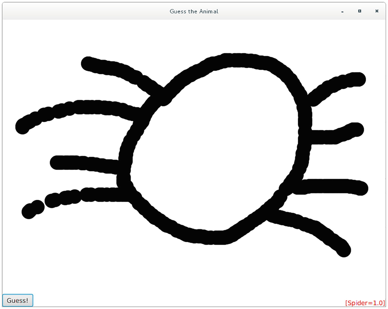
The application can be found in a single class GuessTheAnimal. Running this application results in a screenshot similar to Figure 13-5. The first step is declare constants that contain the input image size, the model location, and the classes we used when we trained the model. In our case, we selected a few animal classes. We used a model with 68% of accuracy and 15 classes. You can use the application from our last section to train your own model and build one with better accuracy:
private static final String MODEL_PATH = "/quickdraw-model-15-68.zip";
A drawing to be analyzed by a LeNet neural network
The application consists of two parts: load the model and build the UI. To load the model, we use the ModelSerializer class. Notice you can use any model exported from the application we discussed before. Just make sure to adjust the constants accordingly. Loading the model is simple. We just need a call to ModelSerializer.restoreMultiLayerNetwork and pass the file or input stream containing the model. See the method initModelAndLoader. In this method, we also create the NativeImageLoader that is the class that will actually do the conversion of the content to an INDArray, making it useful with a neural network:
loader = new NativeImageLoader(INPUT_WIDTH, INPUT_HEIGHT, 1, true);
}
The UI is built in method buildUI(), and it consists of three controls: a canvas used to receive the user’s drawings, a button to trigger the prediction process, and a label that contains the output. When the user drags the mouse on the canvas, the application draws small circles, giving the idea of a pencil writing on a sheet. A right-click cleans the canvas and the result label:
private StackPane buildUI() {
var canvas = new Canvas(APP_WIDTH, APP_HEIGHT);
var btnGuess = new Button("Guess!");
var lblOutput = new Label("");
var root = new StackPane(canvas, btnGuess, lblOutput);
The most important part of this code is where we get the canvas content and convert it to an INDArray so it can be entered in the neural network model. This is done in methods predictCanvasContent and getScaledImage. On getScaledImage, we get a screenshot of the canvas to a WritableImage, convert it to a java.awt.Image using SwingFXUtils, and finally write it to a BufferedImage that also scales the image to the same size of the image used in the neural network model. We also save the last predicted image to an external file; it can be useful for debugging. In predictCanvasContent, we convert the scaledImage to an INDArray that is then input in the neural network model. The model itself returns an INDArray that has 1 × 15 positions; hence, after the prediction, we convert it to a map and filter the result that had results below the threshold we defined as a constant (by default 0.1):
BufferedImage scaledImg = new BufferedImage(INPUT_WIDTH, INPUT_HEIGHT, BufferedImage.TYPE_BYTE_GRAY);
Graphics graphics = scaledImg.getGraphics();
graphics.drawImage(tmp, 0, 0, null);
graphics.dispose();
try {
File outputfile = new File("last_predicted_image.jpg");
ImageIO.write(scaledImg, "jpg", outputfile);
} catch (IOException e) {
e.printStackTrace();
}
return scaledImg;
}
Detecting Objects in a Video
For the next application, we will explore a neural network model architecture called YOLO (You Only Look Once). A summary of how YOLO works can be found in its paper:1
We reframe object detection as a single regression problem, straight from image pixels to bounding box coordinates and class probabilities. Using our system, you only look once (YOLO) at an image to predict what objects are present and where they are.
The paper also brings the following image that simplifies how it works.
The original paper is from 2016. Later, more papers were introduced. The latest one is for YOLO3, which is more precise and faster. Training a YOLO neural network would require bigger images than usual; the input size for the first YOLO version is 448 × 448, which means that it would take a long time in a personal computer. Luckily, DL4J provides TinyYOLO and YOLO2, ready for our use. In this section, we explore a JavaFX application used to detect objects in a running video.
The application starts declaring a few constants important for the application. Let’s go through each constant:
private static final double APP_WIDTH = 800;
private static final double APP_HEIGHT = 600;
private static final String TARGET_VIDEO = "/path/to/video";
TARGET_VIDEO: The URL to a supported video file. If it is in the classpath, you can use the path to it directly; however, JavaFX also supports URL protocol, so local files can be loaded using protocol file:/{path to file}.
THRESHOLD: The cut value. Objects detected with value less than THRESHOLD will not be in the neural network output.
LABELS: The labels used to train the neural network model. By default it has the classes used to train the DL4J default model, but it is possible to change it to a custom YOLO model.
INPUT_WIDTH, INPUT_HEIGHT, INPUT_CHANNELS: The input image information used by the YOLO neural network. It is also using the values for the YOLO2 DL4J model.
GRID_W and GRID_H: The original image is divided in a grid, and the output-detected object positions are related to this grid; hence, when calculating the output box, it is required to use the grid size. It can be calculated using org.deeplearning4j.zoo.model.helper.DarknetHelper getGridWidth and getGridHeight methods.
FRAMES_PER_SECOND: The number of frames scanned by second. If higher, the processing will be longer, but the detected object highlight will look more precise.
The application UI is composed of a media view for the video playback, a pane that will hold the rectangles that will highlight the detected objects, and a label to show the progress of the running task execution. Everything is stacked on StackPane, and the Label is oriented to be on the bottom. This is all done in the start method, but before building the UI, we generate colors for each rectangle that will highlight the detected object and initialize the YOLO2 model. Notice that the first time this code is executed, it will download the pretrained model; hence, it may take a while:
The application also allows users to pause the video by clicking it, and since we have a pane on top of the media view, we register the mouse listener on the pane and not on the media view:
The prediction is not done in real time. The reason is that a single prediction takes almost 500 ms in a machine without GPU processing. When having GPU, part of the prediction process will be done by the multiple GPU cores, making it much faster. The YOLO paper talks about 155 frames per second; however, this result will hardly be achieved taking a snapshot of a JavaFX node, but in this application, snapshot is used because you can preprocess the media view node and only then run YOLO (e.g., zoom or apply effects), uniting the power of JavaFX with YOLO. Also, you may not want to run YOLO on a video. Any JavaFX node can be subject of a YOLO prediction, so it is open for more possibilities.
The trick in our case is not make the prediction in real time, but collect frames when the application is running and schedule a prediction task, create the JavaFX nodes that will contain the detected object highlight, and then display it on top of the video. Notice that once the group is created, we give it an ID so we can hide or show it according to the current frame that is being displayed for the user. We track each task to avoid redundant execution, and a group with the detected object is added to the pane only after the task is finished (see target.setOnSucceeded). In other words, the video needs to play at least one time so all frames are collected and scheduled to be processed. The scheduled tasks are tracked in trackTasks, and once a task for a given frame ID is done, we show the group that contains the detected object highlight and hide the others. Everything is done in a listener attached to the current time of the media player playback, so it is invoked only when the video is playing; otherwise, it won’t collect frames for processing:
var finishedTasks = new AtomicInteger();
var previousFrame = new AtomicLong(-1);
mp.currentTimeProperty().addListener((obs, o, n) -> {
if(n.toMillis() < 50d) return;
Long millis = Math.round(n.toMillis() / (1000d / FRAMES_PER_SECOND));
final var nodeId = millis.toString();
if(millis == previousFrame.get()) {
return;
}
previousFrame.set(millis);
trackTasks.computeIfAbsent(nodeId, v -> {
var scaledImage = getScaledImage(view);
PredictFrameTask target = new PredictFrameTask(yoloModel, scaledImage);
target.setOnSucceeded(e -> {
var detectedObjectGroup = getNodesForTask(nodeId, target);
Now that you understand how we collect frames and process them, let’s think about the actual frame processing. Before scheduling the task, there’s a call to getScaledImage, whose result will be passed to the task. This method gets a snapshot of the media view just like we did before, but this time we are not getting a black-and-white image, but a colored one. YOLO input images use three channels, one for each color (red, green, and blue):
BufferedImage scaledImg = new BufferedImage(INPUT_WIDTH, INPUT_HEIGHT, BufferedImage.TYPE_INT_RGB);
Graphics graphics = scaledImg.getGraphics();
graphics.drawImage(tmp, 0, 0, null);
graphics.dispose();
return scaledImg;
}
On the setOnSucceeded listener, we will then process the detected objects returned by the task. Each object has the initial points for each detected rectangle and also other information, but only points xs are required to build a rectangle to highlight the detected object. However, the coordinates are needed to be transformed before creating our rectangle. First, we need to figure it out if a scale is needed because the app size may be bigger than the image input and all coordinates are relative to the input, then calculate the actual coordinates on the original image because all the coordinates are relative to the grid, and finally calculate the rectangle width and height. Along with the rectangle, we also add a label to show the class that was predicted, and it is added to a group, so we can handle both label and rectangle uniquely. This is done for each detected object:
private Group getNodesForTask(final String nodeId, PredictFrameTask target) {
try {
var predictedObjects = target.get();
var detectedObjectGroup = getPredictionNodes(predictedObjects);
detectedObjectGroup.setId(nodeId);
detectedObjectGroup.setVisible(false);
return detectedObjectGroup;
} catch (Exception e) {
throw new RuntimeException(e);
}
}
private Group getPredictionNodes(List<DetectedObject> objs) {
Finally we have the task, which implements javafx.concurrent.Task and gives it a type of List<DetectedObject>. The JavaFX concurrent task allows us to run some heavy action and later retrieve the result, not holding the main JavaFX thread. The prediction is almost the same thing as done in our Quick, Draw! example. The main difference is that to extract the object, now we use a utility method that is in the org.deeplearning4j.nn.layers.objdetect.Yolo2OutputLayer class to get the predicted objects from the result INDArray:
public class PredictFrameTask extends Task<List<DetectedObject>> {
ComputationGraph yoloModel;
BufferedImage scaledImage;
public PredictFrameTask(ComputationGraph yoloModel, BufferedImage scaledImage) {
This is a very simple starting point to build your own application. Think about the possibilities to build your own YOLO-powered application, like finding invaders in a property, counting the number of cars on a street, looking for objects in a big image, and so on!