Verlet integration

The third and final class of integration schemes that we'll discuss is called Verlet integration. Originally developed for handling complex and variable molecular dynamics simulations because of its stability properties, the approach is now widely used in game programming and animation.

Verlet integration is employed in so-called Verlet systems to simulate the motion of particles subject to constraints. This technique can be applied to connected structures as in ragdoll physics, forward and inverse kinematics, and even rigid body systems. We do not have space to explore this approach, but we refer you to a very good introduction to the subject in the book Advanced ActionScript 3.0 Animation, by Keith Peters. We mention Verlet systems merely to distinguish them from the Verlet integration scheme because they are sometimes confused: Verlet systems are named as such because they use the Verlet integration scheme. But the scheme itself is completely independent of that modeling approach; in fact, it can be used with any other approach, such as the rigid body dynamics discussed in Chapter 13.

Verlet integration schemes are generally not as accurate as RK4 but, on the other hand, are very efficient in comparison. Let's take a look at two common variants of the method: Position Verlet and Velocity Verlet.

Position Verlet

In the Position Verlet method, also known as the Standard Verlet method, the velocity of a particle is not stored. Instead, the last position of the particle is stored, and its velocity can then be computed as needed by subtracting the last position from the current position and dividing by the timestep.

Just as the explicit Euler scheme can be derived starting from the forward difference approximation of the first derivative, the standard Verlet scheme can be derived from the central difference approximation to the second derivative (see Chapter 3). We won't show the derivation here but only quote the final result:

This equation gives the position at the new timestep in terms of the positions at the previous two timesteps without using the velocity.

If desired, the velocity can be computed from the positions―for example, using backward differencing:

Alternatively you can use the central differencing scheme, because the previous position is also known, to give a more accurate estimate of the velocity:

One problem with the Position Verlet equation as given previously is that it assumes that the timestep is constant. But in general the timesteps in your simulation could be variable. In fact, if you are using Timer or EnterFrame, the timesteps will usually vary slightly. To allow for variable timesteps a modified version of the equation is used:

In this equation, Δt(n) denotes the current timestep, and Δt(n-1) denotes the previous timestep. This form can be called the time-corrected or time-adjusted Position Verlet scheme.

Another potential problem that arises in the implementation of the Position Verlet scheme is the specification of the initial conditions. Because the scheme does not use velocity but the position at the previous timestep, you cannot directly specify the initial velocity together with the initial position as you would normally do. Instead, you need to specify the initial position ×(0) as well as the previous position ×(–1) before the initial position! That might sound like nonsense, but you can actually infer the value of that hypothetical position from the initial velocity by applying the backward difference formula for the velocity given previously. Setting n = –1 in that formula gives the following:

Solving this equation for ×(–1) then gives this:

We can now code up a PositionVerlet() function in ForcerIntegrator as follows:

private function PositionVerlet():void{
        var temp:Vector2D = _particle.pos2D;
        if (_n==0){
                _acc = getAcc(_particle.pos2D,_particle.velo2D);
                _oldpos = _particle.pos2D.addScaled(_particle.velo2D,-dt).addScaled(_acc, dt*dt/2);
                _olddt = dt;
        }
        _acc = getAcc(_particle.pos2D,_particle.velo2D);
        _particle.pos2D = _particle.pos2D.addScaled(_particle.pos2D.subtract(_oldpos), dt/_olddt).addScaled(_acc,dt*dt);
        _particle.velo2D = (_particle.pos2D.subtract(_oldpos)).multiply(0.5/dt);                _oldpos = temp;
        _olddt = dt;
        _n++;
}

Note that we have new private variables _oldpos and _olddt for storing the previous position and the previous timestep. There is also a private uint variable _n that represents the number of timesteps that have elapsed since the last call to that function. As you can see from the code, the first time the function is called, the position ×(–1) is set.

Velocity Verlet

One of the problems with the Position Verlet method is that the velocity estimation is not very accurate. The Velocity Verlet method fixes this, albeit at some cost in efficiency. The Velocity Verlet is the more commonly used version of the two. The scheme equations are these:

Comparing the first equation with the corresponding equation in the Euler scheme shows that we now have an additional term that includes the acceleration. The Euler scheme therefore assumes that the acceleration is zero in the interval of one timestep, whereas the Velocity Verlet method takes into account the acceleration but assumes it is constant during that interval. Perhaps you recall the equation s = ut + ½ at² from Chapter 4. The equation for the position update in the Velocity Verlet is exactly of that form (the displacement is s = ×(n+1) – ×(n)).

Also note that the velocity update equation uses the average of the acceleration at the old and the new timestep rather than the acceleration just at the old timestep. Hence, it is a better approximation of the velocity. For these reasons the Velocity Verlet scheme is more accurate than the Euler scheme, as well as having other nice properties such as greater stability and conservation of energy.

Here is the VelocityVerlet() method in ForcerIntegrator:

Testing the stability and accuracy of the Verlet schemes

You can now run the spring and orbit simulations using the Verlet schemes. You should find that they do quite a good job in both cases. Verlet schemes are stable, but they are less accurate than RK4.

A simple test to illustrate the differences in the accuracy of all the different schemes can be done by performing a simulation for a problem with a known analytical solution, against which the numerical solutions can then be compared. You might recall that we did such a test for the Euler scheme for a projectile simulation back in Chapter 4. Let's do something similar now for all the different schemes.

The files Projectile.as and Projector.as contain the setup code and the simulation code, respectively. Once again we won't show any code listings because you've seen those sorts of things tons of times by now. The main thing is that the Projectile class creates a ball and initializes its position and velocity such that the ball is thrown upward at an angle, and the Projector class extends ForcerIntegrator and subjects the ball to gravity. We have set the timestep at 50 milliseconds, as in the other test simulations.

Run the simulation with different integrators specified in ForcerIntegrator. The code in Projector plots the analytical trajectory as well as the numerically computed trajectory (which, of course, the ball follows). You will find that the time-corrected Position Verlet and all the Euler integrators give a trajectory that deviates slightly from the analytical trajectory (see Figure 14-6). On the other hand, the trajectories predicted using the Velocity Verlet, RK2, and RK4 schemes are so close to the analytical trajectory that they cannot be distinguished. Like RK2, the Velocity Verlet scheme is a second-order scheme. Note that these comparisons are for a specific problem, involving constant acceleration. Different schemes might be more or less accurate with different problems.

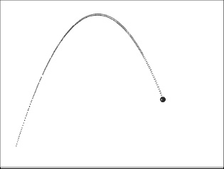
Figure 14-6. Projectile trajectory simulated with Position Verlet scheme (lower curve)

Finally, you might want to check how well the standard Position Verlet does without the time correction. To do this, replace the line of code that updates the position in PositionVerlet() with the following one:

_particle.pos2D =
_particle.pos2D.add(_particle.pos2D).subtract(_oldpos).addScaled(_acc,dt*dt);   

If you then run the code you will find that the simulation gets it completely wrong! The message is that time correction is essential if you have variable timesteps in your simulation.