
Kinematics of uniform circular motion
In Chapter 4, we laid out the framework for describing motion using concepts such as displacement, velocity, and acceleration. As we said there, this framework is technically called kinematics. Those concepts sufficed to describe so-called linear or translational motion. But for analyzing circular or rotational motion, we need additional concepts.
In fact, the concepts of rotational kinematics can be developed in complete analogy with those of linear kinematics. For starters, we have rotational analogs of displacement, velocity, and acceleration that are called angular displacement, angular velocity, and angular acceleration, respectively. So let's start by looking at them.
Angular displacement
Recall that displacement was defined back in Chapter 4 as distance moved in a specified direction. What is the equivalent definition for angular displacement?
First, we need to figure out what concepts are equivalent to distance and direction in rotational motion. Take a look at Figure 9-1, which compares translational motion with rotational motion. On the left, an object moves along a distance d in a given direction. On the right, an object rotates through an angle θ about some center, in a given sense (clockwise in this case). So, it's clear that in rotational kinematics, angle takes the place of distance, and rotation sense (clockwise or anticlockwise) takes the place of direction.
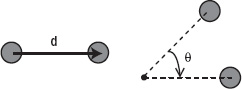
Figure 9-1. Translation and rotation compared for particle motion
Another context in which angular displacement arises is when a rigid body rotates about a fixed axis, as shown in Figure 9-2. In this case, each point on the rigid body moves through the same angle θ about the axis of rotation.
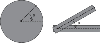
Figure 9-2. Rotation of a rigid body about an axis
In either case (particle rotation about a center or rigid body rotation about an axis), the idea is therefore the same. Hence, we define angular displacement as the angle through which an object moves about a specified center and in a specified sense.
This definition implies that the magnitude of angular displacement is an angle. The usual convention is to use radians for the angle, so we'll do that here.
Angular velocity
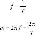
In analogy with linear velocity, angular velocity is defined as the rate of change of angular displacement with time. The usual symbol for angular velocity is ω (the Greek letter omega), so its defining equation in calculus notation is this:
![]()
For a small time interval Δt and angle change Δθ, it can be expressed in this discrete form:
![]()
The latter equation can also be written in the following form:
![]()
This last form of the equation is what we'll use most frequently in code, to calculate the angular displacement due to an angular velocity ω in a time interval Δt.
Angular velocity is measured in radians per second (rad/s) because we divide angle by time to calculate it.
You'll frequently deal with situations where the angular velocity is constant. For example, a particle in uniform circular motion has a constant angular velocity, although its linear velocity is not constant (because its direction of motion changes). Another example is that of an object spinning at a constant rate, such as the Earth.
Angular acceleration
Angular acceleration is the rate of change of angular velocity. It is denoted by the Greek letter α (alpha), and its defining equation is this:
![]()
The definition of angular acceleration implies that it is zero if the angular velocity is constant. Therefore, an object in uniform circular motion has zero angular acceleration. That does not mean that its linear acceleration is zero. In fact, the linear acceleration cannot be zero because the direction of motion (and therefore the linear velocity) is constantly changing. We'll come back to this point a little later in the chapter.
Period, frequency, and angular velocity
Uniform circular motion or rotation is a type of periodic motion (see “Basic Trigonometry” in Chapter 3) because the object returns to the same position at regular intervals. In fact, as discussed in Chapter 3, circular motion is related to oscillatory, sinusoidal motion. Back then, we defined the angular frequency, frequency, and period of an oscillation and showed that they were related by these equations:
The same relationships hold for circular motion, as should be evident by considering Figure 3-16. For circular motion ω is now the angular velocity; it's the same as the angular frequency of the corresponding sinusoidal oscillation. Similarly, f is the frequency of rotation (the number of revolutions per second). Finally, T is the period of revolution (the time it takes to perform one complete revolution).
As an example, let's calculate the angular velocity of the Earth as it orbits the Sun using the formula ω = 2π/T. We know that the period T is approximately 365 days. In seconds, it has the following value:
T = 365 × 24 × 60 × 60 s ≈ 3.15 × 10⁷ s
Therefore the angular velocity has the following value:
ω = 2π/T = 2π/(3.15 × 107) ≈ 2.0 × 10⁻⁷rad/s
This is the angle, in radians, through which the Earth moves around the Sun every second.
Let's now calculate the angular velocity of the Earth as it revolves around its axis using the same formula. In this case, the period of revolution is 24 hours, and so T has the following value:
T = 24 × 60 × 60 s = 86400 s
Therefore, the angular velocity is the following:
ω = 2π/T = 2π/86400 = 7.3 × 10⁻⁵rad/s
Note that this is the angular velocity of every point on the Earth, both on its surface and within it. That's because the Earth is a rigid body so that, as it revolves about its axis, every point rotates through the same angle in the same time. However, different points have different linear velocities. How is the angular velocity related to the linear velocity? Time to find out!
Relation between angular velocity and linear velocity
There is a simple relationship between the linear velocity and angular velocity for an object moving in uniform circular motion. To arrive at this relationship, we first note that the displacement Δs of an object moving through an angle Δθ around a circle of radius r is the length of arc that subtends that angle at the center of rotation. It is therefore given by the following:
![]()
This follows from the definition of the radian given in Chapter 3: one radian is the angle subtended at the center of a circle by an arc of length equal to the radius of the circle. So, by proportion, an arc that makes an angle of Δθ radians at the center must be of length r Δθ (see Figure 9-3).
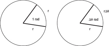
Figure 9-3. Relationship between length of arc and angle at center
Now we can divide this equation on both sides by the time interval Δt for the object to move through that angle:
![]()
But Δs/Δt = v and Δθ/Δt = ω, by definition. Hence, we have the following:
![]()
This formula gives us the linear velocity of an object moving in a circle of radius r at angular velocity ω.
It also applies to a rigid body undergoing rotation about an axis. In that case, it gives the linear velocity at a distance r from the axis of rotation. For a given angular velocity ω, the formula then tells us that the velocity is proportional to the distance from the axis (the farther away you are, the faster is the linear velocity).
Let's apply this formula to the examples discussed in the last section. First, we'll calculate the linear velocity of the Earth in its orbit around the Sun. To work this out, we need to know the radius of Earth's orbit (the distance of the Earth from the Sun): 1.5 × 10¹¹ m. We've already worked out the angular velocity of the Earth in its orbit. It is 2.0 × 10⁻⁷rad/s.
Therefore, the orbital velocity of the Earth is given by the following:
v = r ω = 1.5 × 1011 × 2.0 × 10–7 = 3 × 10⁴ m/s
This is 30 km/s, or 100 000 km/hr. That's about 100 times the typical speed of an airplane!
As a second example, because the Earth's radius is 6.4 × 10⁶ m, and its angular velocity about its own axis is 7.3 × 10⁻⁵rad/s (as we worked out in the last section) the speed of any point on the Earth's surface at the equator due to Earth's rotation has the following value:
v = r ω = 6.4 × 106 × 7.3 × 10–5 m/s ≈ 470 m/s
This is about 1500 km/hr, or about one and a half times the typical speed of an airplane.
Example: A rolling wheel
We now know enough to be able to put together some simple examples. Our first example will be to create rolling wheels. In contrast with most of the examples in the last few chapters, this example will not involve any dynamics, but only kinematics. So we will not compute motion using forces, but will just tell the objects how to move by specifying the velocity directly.
Another difference is that we will code this example up as a standalone piece of code without using the physics library we've been developing. This is partly because we haven't included rotational motion in our physics engine yet and partly as an exercise to make sure we remember the basics.
To begin with, let's create a wheel. We'd like the wheel to look like that shown in Figure 9-4, with an inner and outer rim, and a number of equally spaced spokes (so that we can see it rotating).

Figure 9-4. A rolling wheel
Here is a Wheel class that does the job:
package{

        import flash.display.Sprite;

        import flash.display.Graphics;


        public class Wheel extends Sprite{


                private var _innerRadius:Number;

                private var _outerRadius:Number;

                private var _numSpokes:Number;
                public function Wheel(pIR:Number,pOR:Number, pnumS:Number):void{

                        _innerRadius = pIR;

                        _outerRadius = pOR;

                        _numSpokes = pnumS;

                        drawWheel();

                }


                private function drawWheel():void{

                        with (graphics){

                                beginFill(0);

                                drawCircle(0,0,_outerRadius);

                                endFill();

                                beginFill(0xffffff);

                                drawCircle(0,0,_innerRadius);

                                endFill();

                                lineStyle(4);

                        }

                        for (var n:uint=0; n<_numSpokes; n++){

                                with (graphics){

                                        moveTo(0,0);

                                        lineTo(_innerRadius*Math.cos

(2*Math.PI*n/_numSpokes), _innerRadius*Math.sin(2*Math.PI*n/_numSpokes));

                                }

                        }

                }

        }

}
The constructor of Wheel takes three arguments: the inner radius, the outer radius, and the number of spokes.
Now we'll create a Wheel instance and make it roll. Take a look at the code in WheelDemo.as:
package{

        import flash.display.Sprite;

        import flash.events.Event;


        public class WheelDemo extends Sprite{


                private var _innerRadius:Number=40;

                private var _outerRadius:Number=50;

                private var _numSpokes:Number=10;

                private var _v:Number;

                private var _w:Number=1;         // angular velocity in radians per second

                private var _dt:Number=0.025;    // timestep = 1/FPS

                private var _fac:Number=1;       // slipping/sliding factor


                private var _wheel:Wheel;


                public function WheelDemo():void{

                        init();

                }


                private function init():void{
                        _v = _fac*_w*_outerRadius;        // v = r w

                        _wheel = new Wheel(_innerRadius,_outerRadius,_numSpokes);

                        _wheel.x = 100;

                        _wheel.y = 200;

                        addChild(_wheel);

                        addEventListener(Event.ENTER_FRAME,onEachTimestep);

                }


                private function onEachTimestep(evt:Event):void{

                        _wheel.rotation += _w*_dt*180/Math.PI; // convert w to deg/s

                        _wheel.x += _v*_dt;

                }


        }

}
We created a Wheel instance and then set up an ENTER_FRAME event listener with an event handler onEachTimestep() that increments the rotation and x properties of the wheel at each timestep. This is done using the angular velocity _w and the linear velocity _v by using these formulas:
_wheel.rotation += _w*_dt*180/Math.PI;

_wheel.x += _v*_dt;
The first formula indicates that we are specifying the angular velocity in radians per second; hence the need for the factor 180/Math.PI. The second formula uses the value of velocity _v that is precalculated in the constructor using this formula:
_v = _fac*_w*_outerRadius;
This is basically the formula v = rω, but with an additional factor _fac included to model the effect of slipping or sliding (skidding), with pure rolling if _fac = 1.
Finally, _dt is the timestep that is given the value of 0.025. You may be wondering where that value comes from. This is an estimate of the time interval between successive calls of onEachTimestep(). We expect _dt to be approximately equal to the 1/FPS, where FPS is the frame rate of the movie, which we set at 40. We reiterate that this is just approximate, but is good enough for this simple demo. Recall that in Mover we used the getTimer() function to compute _dt much more accurately.
Run the code with _fac = 1, and you'll see the wheel move so that its translational velocity is consistent with its rotation rate. This gives the appearance of pure rolling without slipping or skidding. If you change the value of _fac to less than 1, say 0.2, the wheel does not move forward fast enough in relation to its rotation; it looks like it's stuck in the mud and is slipping. If you give _fac a value greater than 1, say 5, the wheel moves forward faster than it would do purely as a result of its rotation: it appears to be skidding on ice.
Particles with spin
Before we proceed further, let's update the Particle and Mover classes to allow particles to spin about their center. This is quite straightforward.
In Particle, we create a new property _omega with an associated getter get angVelo() and setter set angVelo() to represent angular velocity:
// angular velocity in radians per second

private var _omega:Number=0;


public function get angVelo():Number{

        return _omega;

}

public function set angVelo(pomega:Number):void{

        _omega = pomega;

}
In Mover, we include an additional protected method spinObject() in the onTimer() function:
private function onTimer(pEvent:TimerEvent):void {

        _dt = 0.001 * (getTimer() - _t0);

        _time += _dt;

        _t0  =getTimer();

        moveObject();

        spinObject();

        pEvent.updateAfterEvent();

}
with spinObject() looking as follows:
protected function spinObject():void{

        if (_particle.angVelo !=0){

        _particle.rotation += _particle.angVelo*_dt*180/Math.PI;

        }

}
This code will make the Particle instance spin on its axis if its angular velocity is non-zero. Note the factor of 180/Math.PI, which converts angles to degrees (because the rotation property deals with degrees rather than radians). A positive value of angVelo will result in a clockwise rotation, and a negative value will result in a counterclockwise rotation.
Any Particle instance animated by a Mover instance will automatically spin if its angular velocity is non-zero. Let's look at a specific example now.
Example: Satellite around a rotating Earth
What we want to achieve in this example is in essence quite simple: an animation of a satellite in a circular orbit around a rotating Earth. The twist is that we want the satellite to orbit so that it is always over the same spot on Earth. This is called a geostationary orbit; as you might guess, it's very useful for telecommunications as well as spying.
Once again, this example will involve only kinematics and no dynamics (no forces). Later on in the chapter, we'll add in the forces.
Let's dive right in and create the setup. We borrow the orbits simulation from Chapter 6 and come up with the following code, in the file SatelliteDemo.as:
package{

        import flash.display.Sprite;

        import com.physicscodes.objects.Ball;

        import com.physicscodes.math.Vector2D;

        import com.physicscodes.objects.Particle;


        public class SatelliteDemo extends Sprite{

                public function SatelliteDemo():void{

                        init();

                }

                private function init():void{

                        // create 100 stars randomly positioned

                        for (var i:uint=0; i<100; i++){

                                var star:Ball = new Ball(Math.random()*3,0xffff00);

                                star.pos2D = new Vector2D(Math.random()*stage.

stageWidth,Math.random()*stage.stageHeight);

                                addChild(star);

                        }


                        // create a spinning Earth

                        var earth:Ball;

                        earth = new Ball(70,0x0099ff,1000000);

                        earth.pos2D = new Vector2D(400,300);

                        earth.angVelo = 0.4;

                        addChild(earth);


                        // create a moving satellite

                        var satellite:Ball;

                        satellite = new Ball(8,0x999999,1);

                        satellite.pos2D = new Vector2D(600,300);

                        //satellite.angVelo = earth.angVelo;

                        // draw antennae

                        with (satellite.graphics){

                                lineStyle(2,0xffffff);

                                moveTo(0,0);

                                lineTo(-20,-10);

                                moveTo(0,0);

                                lineTo(-20,10);

                                moveTo(0,0);

                                lineTo(-15,0);

                        }

                        addChild(satellite);


                        // make the satellite orbit the Earth

                        var orbiter:SatelliteOrbiter=new SatelliteOrbiter(satellite,earth);

                        orbiter.startTime(10);
                        // make the Earth spin

                        earth.move();

                }

        }

}
Most of the code will look familiar. We create some stars, an Earth and a satellite, all as Ball instances. The masses that are given to the various objects are irrelevant here as there is no dynamics. You can put any value you want and the animation will behave in exactly the same way.
In addition, we give the Earth a non-zero angular velocity. We also draw three lines on the satellite to give it a nice old-fashioned, Sputnik-like appearance. Then we make the satellite move with the help of the SatelliteOrbiter class, to be described shortly. Finally we make the Earth spin by the move() method.
The SatelliteOrbiter class is simpler than you might expect. Here is the full code:
package {

        import com.physicscodes.motion.Mover;

        import com.physicscodes.objects.Particle;

        import com.physicscodes.math.Vector2D;


        public class SatelliteOrbiter extends Mover{

                private var _orbiter:Particle;

                private var _omega:Number;

                private var _r:Number;

                private var _x0:Number;

                private var _y0:Number;


                public function SatelliteOrbiter(porbiter:Particle,pattractor:Particle):void{

                        _orbiter = porbiter;

                        _r = _orbiter.pos2D.subtract(pattractor.pos2D).length;

                        _omega = pattractor.angVelo;

                        _x0 = pattractor.xpos;

                        _y0 = pattractor.ypos;

                        super(porbiter);

                }


                override protected function moveObject():void {

                        _orbiter.pos2D = new

Vector2D(_r*Math.cos(_omega*time)+_x0,_r*Math.sin(_omega*time)+_y0);

                }


        }

}
The first thing to note is that SatelliteOrbiter extends Mover instead of Forcer ( as we've been doing most of the time). That's because we are not going to have any forces here. The SatelliteOrbiter constructor takes as arguments an orbiter particle (the satellite) and an attractor particle (the Earth). Although we are using the words orbiter and attractor, we will not model any actual gravitational forces between the particles. Hence, the nature of the animation is different from that of the orbits simulation of Chapter 6. In the constructor, the satellite particle is assigned to a private variable _orbiter, and the distance of the satellite from the Earth is computed and stored in the variable _r. This distance does not change because the orbit will be circular. Then the angular velocity, and x and y position of the Earth are stored in the private variables _omega, _x0 and _y0, respectively.
The action takes place in the overridden moveObject() method, with a single line of code. All we are doing here is telling the satellite where it must be at any time, using these formulas:
![]()
You might recall from Chapter 3 that using cos and sin in this way produces circular motion with angular frequency ω at a radius r. Adding x0 and y0 (the coordinates of the center of the Earth) makes the satellite orbit the Earth. The other important thing is that ω is chosen to be equal to the angular velocity of the Earth. This makes the satellite orbit the Earth at exactly the same rate as the Earth spins on its axis. Run the simulation, and you'll see that this is indeed the case.
We can improve the animation by adding the following line of code to SatelliteDemo.as to make the satellite's antennae always point toward the Earth (see Figure 9.5):
satellite.angVelo = earth.angVelo;
All this line does is to assign the Earth's angular velocity to the satellite's angVelo property, so that it spins in sync with the Earth.
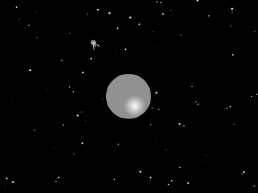
Figure 9-5. A spy satellite orbiting the Earth
The alert reader will have noticed that we've called this example an animation rather than a simulation. That's because we basically told the satellite how to move, rather than prescribing the forces that act on it and letting them determine the motion of the satellite. Although the animation does have some physics realism, it is not totally realistic. One reason is that we have forced the satellite to orbit the Earth at the same rate (the same angular velocity) as the Earth spins around its axis. You can change the distance of the satellite from the Earth's center and it will still orbit at the same rate. In reality, satellites can only do so at a specific distance from the Earth's center; in other words, all geostationary satellites must be at the same distance from the Earth! It is not obvious why that should be so, but the next section will help clarify that and help you to build this feature into the animation.