CHAPTER 5

State Courts

THIS CHAPTER AND THE NEXT CHAPTER examine how a state’s colonial legal system and levels of political competition in the state legislature shaped the independence of judges on the state high court. Figure 5.1 illustrates the basic relationships.

The independence of judges in state high courts influences their behavior on the bench and thus economic and social outcomes. Using a sample of almost all state supreme court cases from 1995 to 1998, Shepherd (2009) found that judges facing Republican electorates in partisan reelections were “more likely to vote for businesses over individuals, for employers in labor disputes, for doctors and hospitals in medical malpractice cases, for businesses in products liability cases, for the original defendant in torts cases, and against criminals in criminal appeals.”¹ Judges facing Democratic electorates had the opposite voting patterns. A variety of other studies examining different time periods and data sets have reached similar conclusions.²

Recent scandals have highlighted the long-standing problems associated with electing high court judges. Getting elected is expensive and requires the support of wealthy donors. These donors, not surprisingly, expect something in return. A detailed study of Ohio by the New York Times in 2006 suggests that donors were getting something. In split-decision cases involving contributors over the period 1994–2006, six of the ten state supreme court judges sided with contributors at least 70 percent of the time. Ohio Supreme Court justice Paul Pfeifer commented, “I never felt so much like a hooker down by the bus station in any race I’ve ever been in as I did in a judicial race. Everyone interested in contributing has very specific interests. They mean to be buying a vote.”³ The problem is not new—getting elected always required having well-positioned supporters, and these supporters always expected something in return for their support.

A theory based on Landes and Posner (1975) and more formally modeled by Maskin and Tirole (2004) and Hanssen (2004b) links levels of political competition in the state legislature to judicial independence. The intuition of the model is straightforward. When political competition is weak, the majority party in a legislature prefers judicial elections. Elections allow the majority party to put political pressure on judges to behave in ways preferred by the majority party. When political competition is strong, the majority party may become the minority party in a future election. In this case, the majority prefers to appoint judges, because they are likely to make favorable rulings in the future if a new majority party emerges.

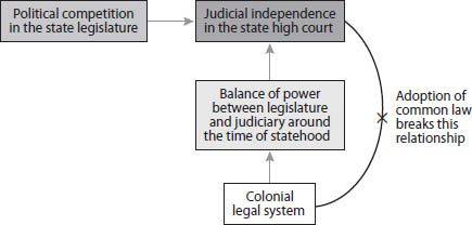
Figure 5.1. Relationships among Legal Initial Conditions, Political Competition, and State Courts.

Independence of state high court judges has been highly persistent. The model provides an explanation for this persistence. Changes will only be made to judicial retention procedures if there are substantial changes in the levels of political competition in the state legislature. In the absence of changes in the levels of political competition, current levels of judicial independence will persist.

Drawing on chapter 2, the model is extended to allow civil-law and common-law legislatures to differ in the benefits they receive from more independent judges. If the benefits to civil-law legislatures of judicial independence are lower, the threshold level of political competition at which they will increase judicial independence will be higher. It is worth noting that for twelve of the thirteen civil-law states shown in figure 5.2, the adoption of common law arguably broke the direct link between the colonial legal system and state courts. The remaining state—Louisiana—poses a problem, because it has not adopted common law. Therefore, our analysis of state courts excludes Louisiana.

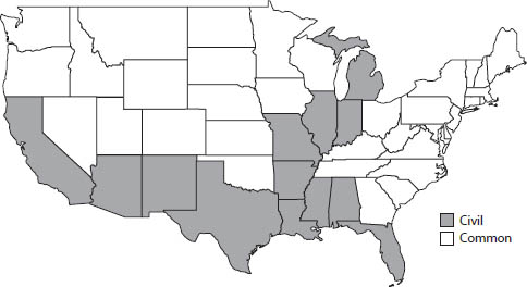
Figure 5.2. Colonial Legal System.

Empirically, civil-law and common-law states have differed in ways predicted by the theory. Civil-law states had lower levels of judicial independence than common-law states, even when controls are included for the timing of the entry of the state into the union and for slavery and when alternative measures of civil law are used. Moreover, civil-law states increased judicial independence at higher levels of political competition than common-law states.

Civil-law states also differed from common-law states in their adoption of intermediate appellate courts. Intermediate appellate courts allow better monitoring of lower-court judges, because many more cases can be reviewed. Under civil law, judges are generally monitored much more closely than under common law. Consistent with this pattern, civil-law states adopted intermediate appellate courts at much lower population levels than common-law states.

JUDICIAL SELECTION AND RETENTION

One of the most important structural features of a state court system is how the supreme court justices are selected and retained. The focus here is on supreme court justices for two reasons. State supreme court justices ultimately hear the most difficult and important state-court cases. Further, judges on the next lower tier of state courts are often selected and retained in the same way as state high court judges.

The relative importance of selection and retention for judicial behavior is the source of some debate.⁴ In practice, it may be difficult to separate the effects of the two, because selection and retention mechanisms tend to be highly correlated. For example, judges who are selected in elections will almost always be retained through elections. We will follow most of the literature and focus on retention procedures. Retention procedures shape the extent to which a judge is free to make decisions without regard to outside pressures. This freedom is often referred to as judicial independence.⁵

Elections tend to offer the least judicial independence, because judges need to be reelected to retain their positions. Under partisan elections, party officials determine whether judges are put on the ballot and control the monetary and nonmonetary resources necessary for reelection. To be reelected, judges have to please both party officials and voters. The need to please these constituents is likely to affect decisions in complicated or controversial cases. Nonpartisan elections are considered to offer somewhat more independence than partisan elections. In general, nonpartisan elections tend to require less cultivation of party officials. In some cases they also require less fund-raising.

Numerous scholars and officials have publicly opposed the election of judges. In a 1906 address to the American Bar Association, the renowned legal scholar Roscoe Pound argued that “putting courts into politics and compelling judges to become politicians in many jurisdictions . . . [has] almost destroyed the traditional respect for the bench.”⁶ The American Bar Association is on record as opposing both partisan and nonpartisan judicial elections. “The American Bar Association urges state, territorial, and local bar associations in jurisdictions where judges are elected in partisan or non-partisan elections to work for the adoption of merit selection and retention.”⁷

Retention elections and appointment-based systems are generally thought to offer considerably more judicial independence. In a retention election, judges run unopposed. Voters vote yes or no on questions that effectively ask: “Should Judge X be retained?” Judges are almost always retained.⁸ The highly politicized and publicized failure of three California Supreme Court justices to be retained in 1986 made it clear that retention elections carry some risk. Appointment-based systems also offer some risk that a judge will not be reappointed, particularly if there has been a change in the party in power or if the court has made one or more very unpopular decisions. In both cases, however, the risk tends to be low relative to the risk associated with elections.⁹

Other features of the court system, such as term length, also affect judicial independence. Judges with longer term lengths are relatively more insulated than judges with shorter term lengths. They can make unpopular decisions early in their career and have time to recover. Depending on their age when they move onto the supreme court, they may choose not to pursue a second term.

Judicial retention procedures vary across states and have varied at the state level over time. The standard narrative divides historical trends in the election and retention of judges into four periods.¹⁰ During the earliest period (1790–1847), all judges were appointed by the legislature or governor or the two acting jointly. This retention process reflected a number of factors, including the primacy of early legislatures, a lack of distinction between lawmaking and judging, and a distrust of colonial judges, many of whom had been loyal to the Crown.

During the second period (1847–1910), states adopted partisan elections in response to the perceived need for state courts to be independent of state legislatures. Based on case studies of four states, Kermit Hall (1987) found that “From the outset, popular election of judges was a lawyers’ reform, one in which politically active lawyers in California and elsewhere dominated the constitutional conventions that adopted partisan elections. These lawyers conceived of election as a means of upgrading the judiciary—and the entire legal profession—by providing it with a base of popular support.”¹¹ Twenty of the twenty-nine existing states and all seventeen of the new states adopted partisan elections. Unfortunately, partisan elections forced judges to participate in the same processes as other political actors, leading to many of the same problems.

In the third period (1910–1958), states tried to reduce the politicization of the judiciary by adopting nonpartisan elections. Seventeen of the forty-six existing states and one of the two new states adopted nonpartisan elections. Although nonpartisan elections were perceived to be an improvement, many citizens felt that judges were still inadequately insulated from the political process. This was the case, for example, in Missouri in the 1930s, where the abuses of the state court system by “Boss Tom Pendergast” in Kansas City and ward bosses in St. Louis led to intense public backlash.¹²

In the fourth period (1958–present), states moved to a system of unopposed retention elections, coupled with merit selection of judges. In 1940 Missouri introduced a merit system for many judges, including state supreme court justices.¹³ Under the “Missouri plan,” a nonpartisan and expert commission selected candidates for a judicial vacancy based on merit.¹⁴ Once the selected candidate finished his or her term, he or she stood for uncontested retention election. The next adoption of the Missouri plan did not occur until 1958, when Kansas made the switch. By 1990, fourteen of the forty-eight continental states had both merit selection and retention elections, and three additional states had other methods of selection coupled with retention elections.¹⁵

It is worth noting that the American Bar Association was not entirely a disinterested party to adoption of the merit system. Lawyers have benefited from the merit systems in two ways. They typically have greater input into who becomes a judge than under other systems. Further, because independent judges are less predictable, it is more worthwhile to file cases than it was when judges were more predictable. In states that adopted merit plans, Hanssen (2002) found that the number of cases filed in state supreme courts increased by 18–32 percent following adoption.

As was discussed in the introduction, different methods of retention appear to have affected judicial behavior. Whether this holds before the 1970s is an open question, because so little work has been done on the earlier period. Shugerman (2009) examined judicial response to the Johnstown flood of 1889, which killed 2,000 people. The flood occurred when heavy rain led to the collapse of a poorly maintained dam. Under the prevailing doctrine, the owners of the dam were not strictly liable for the disaster. Elected judges tended to adopt strict liability for “unnatural activities” quite rapidly after the flood, while appointed judges were much slower. Shugerman argues that the response of elected judges was in part due to selection effects. The election process tended to filter out elite professionals and simultaneously attract lawyer-politicians. The latter tended to be much more responsive to public opinion. He also finds evidence suggesting that term length affected judges’ response to the disaster. Elected judges who had shorter terms needed to please a variety of constituents, including special interests and party officials. Elected judges with longer terms tended to be the most responsive to public opinion. Although they were not required to take action, their backgrounds as lawyer-politicians led them to adopt strict liability.

A MODEL OF STATE LEGISLATURES AND STATE COURTS

A line of work that stretches back to Landes and Posner (1975) and has been developed more fully by Epstein, Knight, and Shvetsova (2002), Maskin and Tirole (2004), and Hanssen (2004a) argues that changes in judicial retention systems are related to changes in levels of political competition. Hanssen (2004b) provides a model of how political competition influences judicial retention. This section incorporates civil law into Hanssen’s model. Since the general intuition has already been discussed in the introduction, readers can skip this section without missing the general argument.

Consider a world with three periods denoted 0, 1, and 2. In periods 0 and 1, Party A is the majority party in the legislature. At the end of period 1 there are legislative elections. Party A wins the election with probability x > 0.5, and Party B wins with probability 1 − x. The party that wins at the end of period 1 is the majority party in period 2.

In period 0, Party A chooses a system of judicial elections or appointments. Appointed judges are guaranteed a job for periods 1 and 2. Elected judges have a job in period 1 and, if reelected, in period 2. If the elected judge loses after period 1, the majority party in period 2 picks a new judge, who then makes a ruling.

In period 1 and in period 2, a judge rules either “a” or “b.” Party A receives a payoff equal to 1 when a judge rules “a” and a payoff equal to 0 when a judge rules “b.” Party B has a completely different agenda and receives a payoff of 1 when a judge rules “b” and a payoff of 0 when a judge rules “a.”

At the beginning of period 1, Party A picks a judge, where δ > 0.5 is the probability that the chosen judge prefers ruling “a”; δ can be thought of as representing a party’s ability to screen for judges who will behave in the way that the party prefers. The judge then makes a ruling that is observed at the end of the period. Suppose that the judge is elected. If the incumbent party, Party A, wins the election and the judge rules “a” in period t = 1, that judge remains in office. If Party A wins and the judge rules “b” in period 1, the judge is removed, and Party A picks a new judge at the start of period t = 2. If Party B wins, the judge keeps her job in period 2 only if she ruled “b” in period 1. Since x is the probability that Party A remains in office in period 2, our measure of political competition, denoted pc, is 1 − x.

There are two kinds of judges, and their preferences are common knowledge. Let P denote the payoff to a judge who makes her preferred ruling in period 1, and let O denote her payoff from holding onto her office during periods 1 and 2. If judges are elected and O > P, then the judge makes ruling “a” in period 1 and makes her most preferred ruling in period 2. In this case, the legislature’s threat of being able to remove her from office gets the judge to make ruling “a” in period 1 even when “b” is her preferred ruling. If O < P, the judge makes her preferred ruling in period 1 even if this means she loses her job. In period 2, a judge makes her preferred ruling. Setting up a simple game tree, it is straightforward to show Party A’s payoffs associated with elections when O < P and O > P are

V, elections (if O < P) = δ(2 + x − δ)
V, elections (if O > P) = 1 + xδ + (1 − x)(1 − δ).

Now suppose that civil-law legislatures experience disutility from an independent judiciary, denoted c, where 0 < c < 1. Then it is straightforward to show that Party A’s payoffs from a system of appointments when it operates in a common-law and civil-law state are

V, appointed (common) = 2δ
V, appointed (civil) = 2(δ − c).

Using these payoffs, critical levels of political competition can be computed, pc* = 1 − x*, for common-law and civil-law legislatures.

Suppose O < P, which means that elected judges make their most preferred ruling, even if this costs them their job. Thus, for common-law states, the critical level of political competition is pc*(common) = 1 − d. For civil-law states, it is pc*(civil) = 1 + 2c − δ. Civil-law legislatures require a higher level of political competition before they switch to an appointment system. If screening is sufficiently precise (δ is close to unity), common-law states would almost always prefer appointments, and political competition will be less important as a force for removing elections.

Suppose that O > P, which means elected judges make the ruling “a” in period 1 so that they can stay in office. Then, pc*(common) = (1 − δ) / (2δ − 1) and pc*(civil) = (1 − δ + 2c) / (2δ − 1). Again, civil-law states require higher political competition to make changes.

If screening is assumed to be constant across states, the model implies that for any political history where the maximum level of political competition for all states is below pc*(common), all states will have elections. Similarly, for any political history where the maximum level of political competition for all states is above pc*(civil), all states will have elections. In the interval pc*(common) to pc*(civil), common-law states will appoint their judges, and civil-law states will elect their judges.

It is worth noting two other things about the model. Although the discussion focuses on how increases in political competition will cause states to switch from elections to appointment, the reverse can also happen. That is, declines in political competition can lead states to switch from appointment to elections. The model also implies that if political competition in a state varies around pc*, a state might switch frequently, possibly in every period. In practice, changes in judicial retention procedures for high court judges involve changing the state constitution, which is time consuming and costly. So states are unlikely to make frequent changes to judicial retention procedures. Indeed, most states have made between zero and two changes to judicial retention procedures over the course of their history.

POLITICAL COMPETITION, CIVIL LAW, AND JUDICIAL RETENTION

Table 5.1 presents summary statistics for judicial retention systems and political competition. The average value of partisan elections was 0.46, the average value of judicial independence was 2.9, and the average term length was 9.6 years, and the average value of the Ranney index was 52. The coding of judicial independence is from to Epstein, Knight, and Shvetsova (2002). Their index runs from 1, which is partisan elections and low judicial independence, to 9, which is life tenure and high judicial independence.¹⁶ It tries to capture the opportunity cost of a judge acting on his beliefs in a potentially controversial case. Judges with higher opportunity costs have lower scores and less judicial independence.

TABLE 5.1.
SUMMARY STATISTICS FOR JUDICIAL RETENTION AND POLITICAL COMPETITION

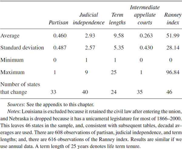
Table 5.2 shows the correlations among judicial retention systems, political competition, and colonial legal system. Use of partisan elections was negatively correlated with the Ranney index and positively correlated with civil law. Judicial independence was negatively correlated with civil law and relatively uncorrelated with the ranney index. Term length was weakly positively correlated with the Ranney index and weakly negatively correlated with term length.

TABLE 5.2.
CORRELATIONS FOR JUDICIAL RETENTION AND POLITICAL COMPETITION

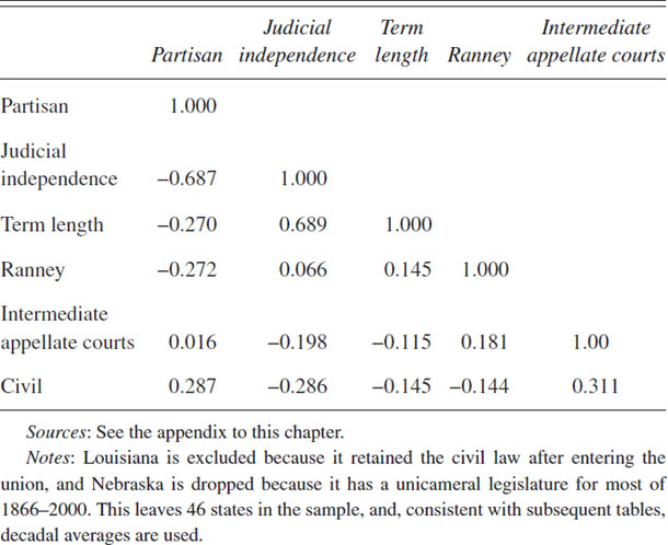
Figure 5.3 shows that levels of judicial independence were highly persistent over time. States with higher levels of judicial independence in 1900–1918 had higher levels of judicial independence from 1866 to 2000. This is striking and suggests that levels of judicial independence were set very early on.

The model predicts that the threshold levels of political competition above which states will change their retention methods will differ in civil-law and common-law states. This implies that civil-law states will, controlling for the level of political competition, be more likely to use partisan elections and have lower judicial independence than common-law states.

Figure 5.4 illustrates how the evolution of political competition was related to the evolution of partisan election systems. Recall that partisan elections were widely considered to be good for the quality of courts through at least 1900. The model predicts that partisan elections will be removed when political competition is sufficiently high. The trends starting in the mid-1920s are consistent with this prediction.

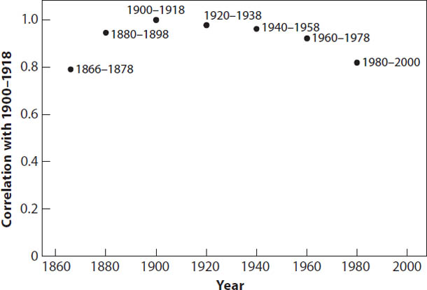
Figure 5.3. Persistence of Judicial Independence in State High Courts’ Judicial Independence, 1866–2000.

The judicial independence index runs from 1 (partisan elections and least independent) to 9 (lifetime tenure and most independent). This index was constructed by Epstein, Knight, and Shvetsova (2002) and is discussed in detail in chapter 5. Louisiana is excluded because it retained civil law after entering the union and Nebraska is dropped because it has a unicameral legislature for most of 1866–2000. Eleven additional states are dropped for lack of data. This leaves 35 states in the sample. The results are similar if we include these 11 states and conduct the analysis for 1910–2000.

Figure 5.5 confirms that common-law and civil-law states differed systematically in their use of partisan elections. Civil-law states adopted partisan elections more rapidly than common-law states during the nineteenth and early twentieth centuries. Civil-law states that had partisan elections moved away from them more slowly during the twentieth century than did common-law states.

Why would civil-law states have been so enamored with partisan elections and elections more generally? Following the French Revolution, the French briefly considered using partisan elections to retain judges. Ultimately, judges were made part of a bureaucracy.¹⁷ Both historically and today, French judges, particularly younger judges, are supervised and can be punished for decisions that systematically differ from norms regarding appropriate outcomes. Adherence to the norms is an important factor in promotion within the bureaucracy. Outside options are limited, so the primary path is to rise within the judicial hierarchy. This system is in many ways more restrictive than the American system under partisan elections, because judges are constantly being evaluated and can be sanctioned for poor decision making at any time, not just at the time of reelection.

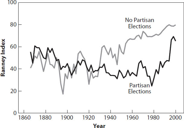
Figure 5.4. Political Competition and Partisan Elections, 1866–2000.

Louisiana is excluded because it retained civil law after entering the union, and Nebraska is dropped because it has a unicameral legislature for most of 1866–2000. This leaves 46 states in the sample. Sources: See the appendix to this chapter.

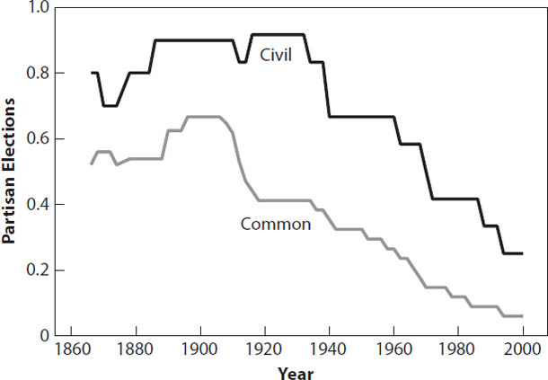
Figure 5.5. Use of Partisan Elections for High Court Judges by Common-Law and Civil-Law States, 1866–2000.

The vertical axis is the share of states that use partisan elections. Louisiana is excluded because it retained civil law after entering the union, and Nebraska is dropped because it has a unicameral legislature for most of 1866–2000. This leaves 46 states in the sample. Sources: See the appendix to this chapter.

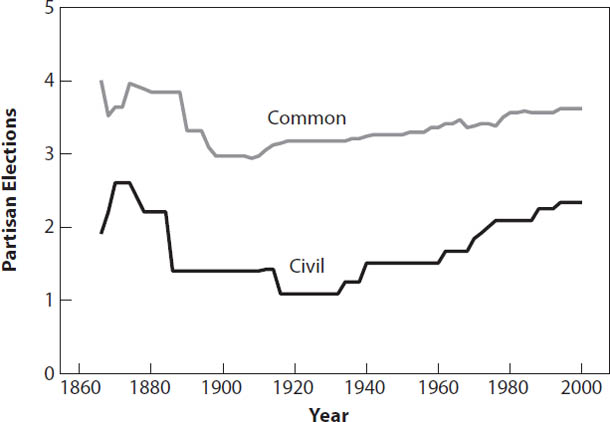
Figure 5.6. Epstein et al. Measure of Judicial Independence, 1866–2000.

The Epstein, Knight, and Shvetsova (2002) index runs on a scale of 1 (least independent) to 9 (most independent). The vertical axis is the average score on the Epstein et al. index for civil-law and common-law states. Louisiana is excluded because it retained civil law after entering the union, and Nebraska is dropped because it has a unicameral legislature for most of 1866–2000. This leaves 46 states in the sample. Sources: See appendix to this chapter.

Figure 5.6 documents differences in judicial independence in common-law and civil-law states. Over the period 1866–2000, civil-law states had systematically lower levels of judicial independence than common-law states.

The evidence presented in figures 5.4–5.6 is suggestive but hardly conclusive. Table 5.3 examines the relationships among political competition, colonial legal origins, and judicial retention in a regression framework. Because retention systems change infrequently, measures of Ranney and retention systems are decadal averages.

TABLE 5.3.
CIVIL LAW, POLITICAL COMPETITION, AND PARTISAN ELECTIONS

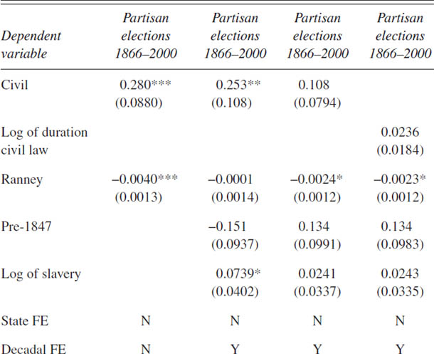
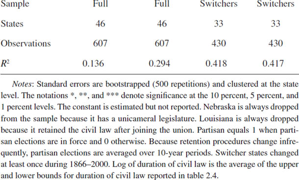
The first column suggests that the basic intuition of the model is correct. States with higher levels of competition in the state legislature were statistically significantly less likely to use partisan elections, and civil-law states were statistically significantly more likely to use partisan elections. The effects of political competition were relatively small. A twenty-point increase in the Ranney index decreased the predicted use of partisan elections by 0.08.¹⁸ the effect of civil law was substantially larger. Civil-law states’ predicted use of partisan elections was 0.28 higher than common-law states’.¹⁹

One concern is that the civil-law variable may be picking up things other than the historical influence of civil law on the balance of power between state legislatures and state courts. For example, since many civil-law states are in the South, civil law could be capturing something related to slavery. Or it could be capturing differences between states that entered before 1847, when all states entered with appointment, and states that entered after 1847, when states entered with partisan or nonpartisan elections.

An important decision with respect to specification is whether to include decadal fixed effects. The model focuses exclusively on the state legislature, but other factors may affect whether a change in retention is likely to occur. For example, outside actors may lobby for change, the governor may or may not support change, and the electorate typically has to ratify the change. Further, the economy and changing views on the appropriate system for judicial retention may also affect change. The inclusion of decadal fixed effects will capture national trends likely to affect changes in retention systems. At the same time, their inclusion poses a much more restrictive test for the importance of the Ranney index, because it will also capture national time trends in the Ranney index.

The remaining columns in table 5.3 include controls. Adding controls has little effect on the civil variable in the second column. The coefficient remains positive, statistically significant and large.

The last two columns restrict the sample to the thirty-three states that changed to or from partisan elections at some point during 1866–2000. In particular this sample excludes Arizona, Arkansas, Connecticut, Delaware, Maine, Massachusetts, New Hampshire, New Jersey, Rhode Island, South Carolina, Vermont, Virginia, and West Virginia. The fourth column replaces civil law with a variable measuring the duration of civil law during the colonial period.²⁰ The effect of civil law on the use of partisan elections falls and becomes statistically insignificant when the sample is restricted to switchers. The coefficient on the Ranney index is small, but statistically significant for switchers, even with the inclusion of decadal fixed effects.

Table 5.4 moves away from partisan elections to focus on judicial independence more broadly. It shows that civil law and entry date are strongly related to judicial independence. Across all four specifications, the coefficient on civil law is negative, statistically significant, and large. Levels of judicial independence in civil-law states were 1.0–1.7 lower than in common-law states. The type of retention system that a state entered with also had an enduring effect. States that entered before 1847 had levels of judicial independence that were 1.5–2.5 higher than states that entered after.²¹ these are large effects, given that the mean level of judicial independence in the sample was 2.9.

Overall, tables 5.3 and 5.4 confirmed that civil-law and common-law states used different methods to retain their state high court judges. Civil-law states were more likely to use partisan elections and had lower levels of judicial independence than common-law states. This is consistent with the predictions of the model.

We test the prediction of the model more directly in table 5.5 by comparing the threshold levels of political competition at which common-law and civil-law states switch. Levels of political competition are included in the two periods preceding the switch, since it may take time for change to occur, conditional on having reached the threshold level of political competition, pc*. Further, the two periods following the switch are included, since the relevant political players may choose to act on change prior to actually reaching pc*. That is, they may forecast reaching pc* in the near future and initiate change while their political power is still strong.

TABLE 5.4.
CIVIL LAW, POLITICAL COMPETITION, AND JUDICIAL INDEPENDENCE

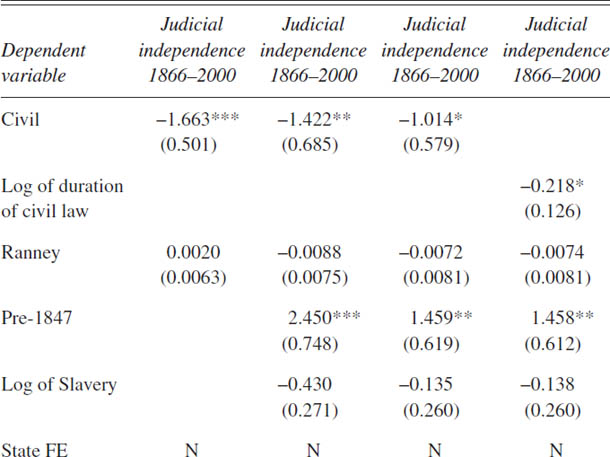
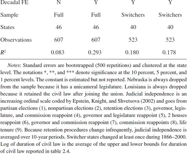
TABLE 5.5.
RANNEY INDEX AT THE TIME OF CHANGES IN JUDICIAL RETENTION

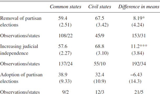
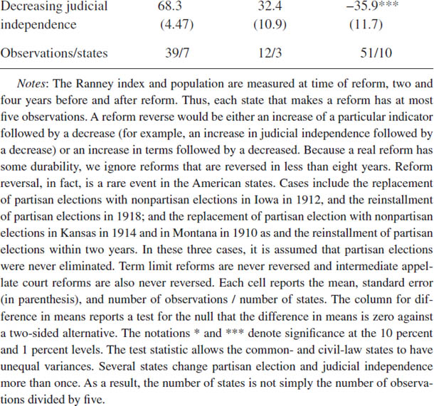
Consistent with the model, civil-law states moved away from partisan elections and increased judicial independence at higher levels of political competition than common-law states. For partisan elections, the average Ranney index was 58 in common-law states and 70 in civil-law states. For judicial independence, the average Ranney index was 59 in common-law states and 71 in civil-law states. In both cases, the differences were statistically significant using a two-sided t-test. The states that adopted partisan elections were southern states that did so in the aftermath of the Civil War. They did so at very low levels of political competition. Six other common-law states decreased judicial independence, and they did so at relatively high levels of political competition. This creates the large differential between common-law states and civil-law states with respect to decreasing judicial independence.

Table 5.6 examines a related prediction of the model. The model implies that changes in judicial retention should be associated with increased political competition in the state legislature. The idea is that an increase in political competition pushes the legislature into a region in which the legislature prefers a more independent judiciary. By extension, this intuition should hold for both common-law and civil-law states. Our model does not, however, have direct implications regarding the relative strength of the relationship in common-law and civil-law states.

Whether the relationship between political competition and the use of partisan elections differs for the two groups of states is explored by estimating the following specification.

Partisan_id = α + β₁Ranney_id + β₂Ranney_id*Civil_i + S_i + ε_id.

partisan_id is the share of state years when partisan elections were in force and the Ranney index in state i in decade d, and Ranney_id is the Ranney index in state i in decade d; Civil_i is an indicator variable for civil law, S_i is state fixed effects, and ε_id is the stochastic error term. β₁ measures the impact of the Ranney index in common-law states, and β₂ measures the differential impact of the Ranney index in civil-law states.

Table 5.6 shows that states removed partisan elections during periods of rising political competition.²² In the first column, a twenty-point increase in the Ranney index decreased the predicted use of partisan elections by 0.12. The second column shows that the relationship is very similar if attention is restricted to states that actually changed their retention system at some point in the period 1866–2000. The third column shows that the relationship between political competition and partisan elections differed in common-law and civil-law states. The difference was, however, modest and not statistically significant. The fourth column yields similar results.

TABLE 5.6.
POLITICAL COMPETITION, CIVIL LAW, AND PARTISAN ELECTIONS WITH STATE FIXED EFFECTS

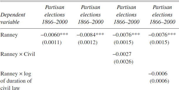
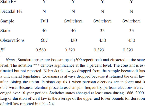
TABLE 5.7.
POLITICAL COMPETITION, CIVIL LAW, AND JUDICIAL INDEPENDENCE WITH STATE FIXED EFFECTS

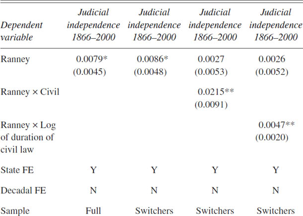
Table 5.7 shows that civil-law states increased judicial independence during periods of rising political competition, whereas common-law states did not. The first two columns are consistent with the results for partisan elections. The third and fourth columns suggest that the effect is primarily due to civil-law states. Common-law states did not generally increase independence during periods of rising political competition.

JUDICIAL TERMS

Longer tenure gives judges greater independence because they face elections or other reappointment procedures less often.²³ Depending on judges’ age at the time of appointment to the state supreme court, if the judicial term is long enough, they may never face reappointment. Like judicial retention systems, there have been historical trends in term length.²⁴ Up until the 1830s high-level judges in most states had life tenure. During the 1840s and 1850s, average term length fell quite dramatically from about twenty years to about ten years, as many states shifted from life tenure to fixed terms. Average term length fell by another year during the remainder of the nineteenth century and averaged about nine years during the twentieth century. This section examines the factors that determined term lengths.

Figure 5.7 suggests that political competition has been related to term length over the period 1866–2000. The differences in levels of political competition in states with terms of less than ten years and states with terms greater than or equal to ten years were around twenty points for much of the period. The difference disappeared around 1980.

Figure 5.8 shows that civil-law states had consistently shorter terms than common-law states. The difference in term lengths was almost three years in the early twentieth century and narrowed to about two years during the late twentieth century.

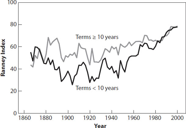
Figure 5.7. Political Competition and Term Length, 1866–2000.

Tenured judges are assigned 25-year terms. Louisiana is excluded because it retained civil law after entering the union, and Nebraska is dropped because it has a unicameral legislature for most of 1866–2000. This leaves 46 states in the sample. Sources: See the appendix to this chapter.

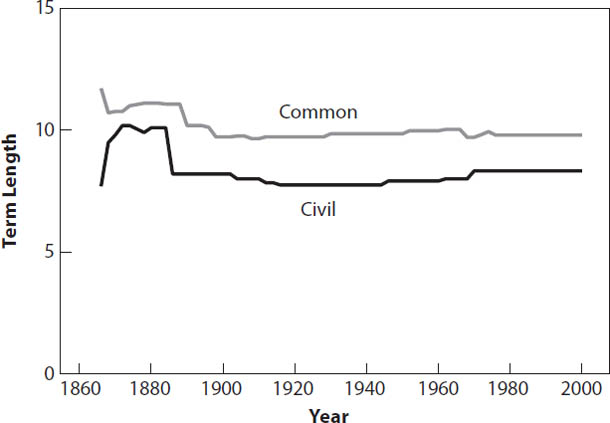
Figure 5.8. Term Length, 1866–2000.

Tenured judges are assigned 25-year terms. Louisiana is excluded because it retained civil law after entering the union, and Nebraska is dropped because it has a unicameral legislature for most of 1866–2000. This leaves 46 states in the sample. Sources: See the appendix to this chapter.

Table 5.8 shows that term length was positively related to political competition. The coefficient on the Ranney index is positive, statistically significant, and large in three of the four columns. For example, in the first column a twenty-point increase in the Ranney index would increase term length by 0.5 years. In the third and fourth columns, a twenty-point increase in the Ranney index would increase term length by 1.1 years. The civil variable is uniformly negative but not statistically significant.

Table 5.9 documents that civil-law states increased term length at higher levels of political competition than common-law states. The differences were large. For term length, the average Ranney index was 56 in common-law states and 86 in civil-law states. The decreases in term length in civil-law states occurred in southern states after the Civil War. Thus, the levels of political competition were very low.

Table 5.10 indicates that term lengths were only weakly related to increases in political competition.

INTERMEDIATE APPELLATE COURTS

Intermediate appellate courts were introduced to allow the review of more cases, given the limited capacity of the state supreme court. Two states—Illinois and Missouri—adopted intermediate courts the 1870s. The pace of adoption was slow, however. In 1948, only eleven states had intermediate appellate courts. As late as 1956, only three more states had intermediate appellate courts. Adoption accelerated in the 1960s, and by 2000, intermediate appellate courts were operating most states.²⁵ Kagan et al. (1978) argued that population growth was a major reason for the emergence of these courts. Population growth created a case overload in state supreme courts. Creating intermediate appellate courts allowed state high courts to control their docket and make careful rulings.

Why would colonial legal origins matter for intermediate appellate courts? Legislatures in civil-law states may have pushed for the adoption of intermediate appellate courts because it improved their ability to control lower courts. Lower courts are difficult to control because the numbers of judges are large and their locations are spread throughout the state. With little prospect for judicial review, these courts have considerable autonomy. By expanding the capacity for oversight in the form of intermediate appellate courts, the legislature can limit this autonomy. Further, since appellate courts are often located in the state capital, where the legislature and supreme court are also located, state legislators can more easily exert pressure on intermediate appellate judges than on the more numerous and geographically dispersed lower-court judges.

TABLE 5.8.
CIVIL LAW, POLITICAL COMPETITION, AND TERM LENGTHS

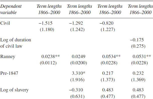
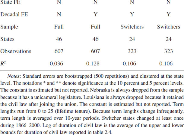
TABLE 5.9.
RANNEY INDEX AT THE TIME OF CHANGES IN TERM LENGTH AND POPULATION AT THE TIME OF ADOPTION OF INTERMEDIATE APPELLATE COURTS

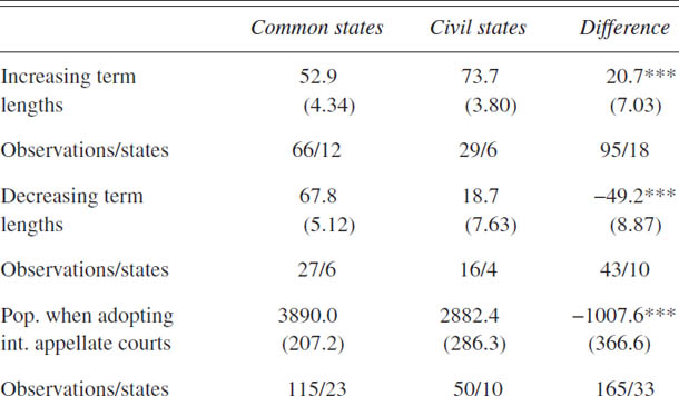
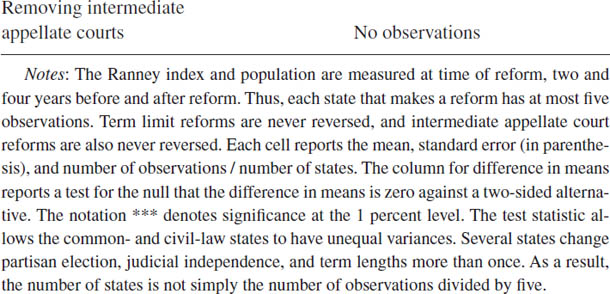
TABLE 5.10.
POLITICAL COMPETITION, CIVIL LAW, AND TERM LENGTHS WITH STATE FIXED EFFECTS

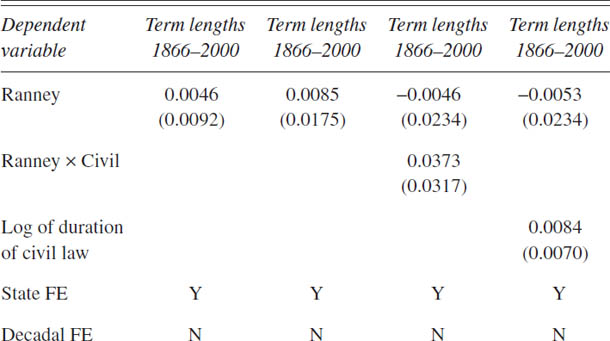
Figure 5.9 illustrates the strong association between population and intermediate appellate courts. The states with intermediate appellate courts were more heavily populated. Moreover, this difference in population between states that had and did not have intermediate appellate courts generally increased over time. In contrast, figure 5.10 suggests that political competition has played little role in the evolution of intermediate appellate courts.

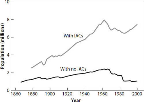
Figure 5.9. Population and Intermediate Appellate Courts, 1866–2000.

Louisiana is excluded because it retained civil law after entering the union, and Nebraska is dropped because it has a unicameral legislature for most of 1866–2000. This leaves 46 states in the sample. Sources: See the appendix to this chapter.

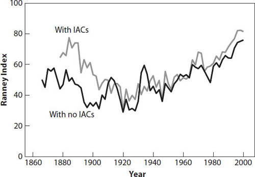
Figure 5.10. Political Competition and Intermediate Appellate Courts, 1866–2000.

Louisiana is excluded because it retained civil law after entering the union, and Nebraska is dropped because it has a unicameral legislature for most of 1866–2000. This leaves 46 states in the sample. Sources: See the appendix to this chapter.

Figure 5.11 indicates that civil-law states adopted intermediate appellate courts more rapidly than their common-law counterparts. By 1920, six of the twelve civil-law states in our sample had intermediate appellate courts. By 2000, all of them had intermediate appellate courts. In comparison, four of the thirty-four common-law states had intermediate appellate courts in 1920. By 2000, twenty-three of the common-law states had had intermediate appellate courts.

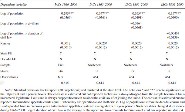
Table 5.11 confirms the importance of both population and civil law for intermediate appellate courts. The coefficients on both variables were statistically significant in all three specifications. The magnitudes of the effects were similar across all three specifications. Civil-law states’ use of intermediate appellate courts was 0.22–0.2 higher than common-law states’. The coefficient on Log of population ranged from 0.16 to 0.21. Table 5.9 indicates that civil-law states adopted intermediate appellate courts at lower levels of population than common-law states.

Table 5.12 shows that states adopted intermediate appellate courts during periods of rising population within states. The differences between civil-law and common-law states in how they responded to increases in population were tiny and not statistically significant.

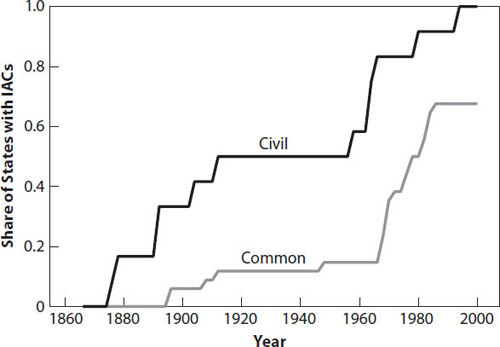
Figure 5.11. Use of Intermediate Appellate Courts, 1866–2000.

The vertical axis is the share of states that have operating intermediate appellate courts. Louisiana is excluded because it retained civil law after entering the union, and Nebraska is dropped because it has a unicameral legislature for most of 1866–2000. This leaves 46 states in the sample. Sources: See the appendix to this chapter.

TABLE 5.11.
CIVIL LAW, POLITICAL COMPETITION, AND INTERMEDIATE APPELLATE COURTS

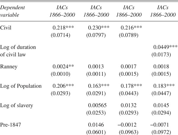
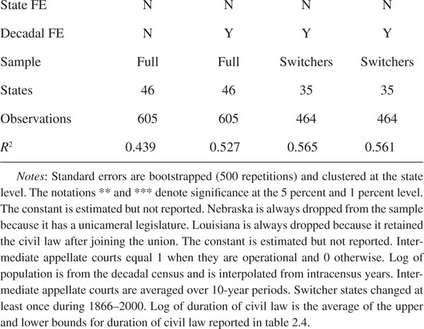
TABLE 5.12.
CIVIL LAW, POLITICAL COMPETITION, AND INTERMEDIATE APPELLATE COURTS WITH FIXED EFFECTS

CONCLUSION

This chapter presented a model of how state legislatures choose judicial retention systems. The model generated predictions regarding the threshold levels of state political competition at which legislatures would change judicial retention procedures. This threshold level will be lower for common-law states than for civil-law states.

Tables 5.3–5.7 documented a number of differences between civil-law and common-law states in judicial retention procedures that were consistent with the model. Controlling for levels of political competition, the two groups of states differed in their use of partisan elections and in their levels of judicial independence. Civil-law states were more likely to use partisan elections and had lower levels of judicial independence than common-law states. Civil-law states made changes to judicial retention procedures at higher threshold levels of political competition than common-law states. As predicted by the model, states made changes during periods of rising political competition.

Other differences not directly related to the model were also documented. Two differences—one related to judicial tenure and one related to intermediate appellate courts—were of particular interest. Tenure of state high court judges was strongly related to state political competition. Civil-law states changed tenure at higher levels of political competition. Controlling for population and political competition, civil-law states adopted intermediate appellate courts earlier than common-law states. This is consistent with politicians in these states having a greater desire to monitor lower court judges than politicians in common-law states.

¹ Shepherd (2009), 188.

² See also Hall (1987, 1992), Tabarrok and Helland (1999), Hanssen (1999), Bohn and Inman (1996), and Huber and Gordon (2004).

³ Liptak and Roberts (2006).

⁴ A number of authors have argued that the judges selected are similar, but they behave differently once on the bench, because of the retention process. Canon (1972), Glick and Emmert (1987), and Besley and Payne (2003) address this issue. Hall (1984) provides evidence that northern and southern judges have similar educational and family backgrounds. Recent empirical work by Choi, Gulati, and Posner (2008) suggests that both may be important. Judges subject to partisan elections were more likely to have gone to in-state and lower-ranked law schools than appointed judges. They argue that elections encourage state judges to behave more like politicians who focus on providing service to their constituents and that appointment to the judiciary encourages judges to behave more like professionals who focus on building a legacy as creators of law.

⁵ See Kornhauser (2002) for a discussion of the concept and its usefulness.

⁶ Pound (1906).

⁷ American Bar Association resolution in 1994, quoted in Cardman (2007).

⁸ See Dubois (1980), Hall (1987), Hall (1995), Brace and Hall (1997), and Bonneau (2005).

⁹ See Dubois (1980) for the period 1948–1974 in nonsouthern states. In table 13, p. 109, he shows that sizeable numbers of incumbents were defeated in some states with elections. Ohio (10), Colorado (6), Michigan (5), New Mexico (5), and Indiana (4) all had sizeable numbers of defeats. Many of these judges were appointed to finish an unexpired term and then were defeated in their first election. See Bonneau (2005) for the period 1990–2000. He finds 39 percent of incumbents were defeated in contested partisan elections and 10 percent were defeated in contested nonpartisan elections. Hall (2001) finds similar results for the period 1980–1995. Hall (1987) finds that over the period 1850–1920 18 percent of California Supreme Court justices were not renominated by their party or were not reelected. During the period from 1879–1900, the rate was 29 percent. Hall (2006) finds that over this same period 20 percent of Ohio Supreme Court justices were defeated at the polls.

¹⁰ See Hanssen (2004a) and epstein, Knight, and Shvetsova (2002).

¹¹ Hall (1987), 65.

¹² See Karlen (1970).

¹³ California adopted retention elections in 1934, but it did not have merit selection. Thus, Missouri is considered to have introduced the first true merit plan.

¹⁴ The governor or the judicial commission selects the final candidate.

¹⁵ The Book of the States (1991). For case studies of change and failure to change, see Becker and Reddick (2003).

¹⁶ Higher numbers correspond to fewer parties being involved in the reappointment process. The coding is partisan elections (1), nonpartisan elections (2), retention elections (3), governor, legislature, and commission reappointment (4), governor and legislature reappointment (5), reappointment by both houses (6), governor and commission reappointment (7), commission reappointment (8), life tenure (9).

¹⁷ See Bell (1988), Volcansek et al. (1996), and Merryman and Perez-Perdomo (2007).

¹⁸ Twenty points is roughly two-thirds of a standard deviation in the Ranney index.

¹⁹ Because the graphs suggest that the effect of the civil variable was relatively constant over time, its effects are estimated as a constant, rather than a time-varying effect. For more on the time-varying effects, see table 5.1A. For most outcomes in most time periods, the coefficient on the civil variable was not statistically significantly different from its value in 1900–1908.

²⁰ Duration of civil law is taken from table 2.4 and is the average of the upper and lower bounds for years of civil law.

²¹ This result would appear to differ from the result in table 5.3. The difference stems in part from differences in the composition of the sample—thirty-three states changed to or from partisan elections, while forty states changed judicial independence. These seven additional states had much higher levels of judicial independence than the thirty-three that changed to or from partisan elections.

²² This table and similar tables that follow do not include decadal fixed effects. Adding decadal fixed effects causes the coefficient on the Ranney index to become statistically insignificant in most specifications.

²³ Choi, Gulati, and Posner (2008) argue that while it increases independence, length of term does not necessarily increase judicial quality.

²⁴ See Epstein, Knight, and Shvetsova (2002). We follow them in assuming life tenure on average is twenty-five years.

²⁵ For more on the modern role of intermediate appellate courts, see Chapp and Hanson (1990).